An Introduction to Mean-Field Langevin Dynamics

Optimization over the space of probability measures is not only widely applicable, but also offers a useful perspective for analyzing certain complicated finite-dimensional nonconvex optimization problems. In particular, lifting such problems to optimization problems over probability measures can lead to better structural properties, such as convexity. Mean-field Langevin dynamics provides a representative example of this idea. Its central motivation is that some highly nonconvex optimization problems arising in neural network training become better behaved when reformulated as the optimization of a functional on the space of probability measures. This viewpoint also makes it possible to build a theoretical foundation for understanding the convergence of SGD. In what follows, we briefly introduce this perspective, mainly based on the paper by [Hu, Kaitong, et al]. The main analytical framework of this theory can be illustrated by Figure 2.

Motivation: Neural Networks

Suppose we have datasets $(z_m,y_m)_{m=1}^N$, where $z_m\in \mathbb{R}^{l_0}$ is the data and $y_m\in \mathbb{R}^{l_L}$ is the corresponding label. The aim of the neural network is to reconstruct the map from all $z_m$ to $y_m$.

Let $\varphi:\mathbb{R}\to\mathbb{R}$ be a nonlinear activation function and $\varphi^l:\mathbb{R}^l\to\mathbb{R}^l$ be pointwise, that is
$$
\varphi^l(z)=(\varphi(z_1),\varphi(z_2),\cdots,\varphi(z_l))\quad \text{for } z=(z_1,z_2,\cdots,z_l).
$$
Then the framework for neural neural network is shown as follows.

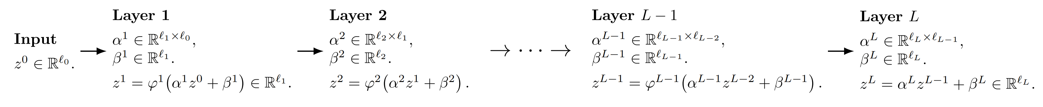Figure 1: The framework for neural neural network.

The parameters we need to optimize can be listed as
$$
\Psi=\left((\alpha^1,\beta^1),(\alpha^2,\beta^2),\cdots,(\alpha^L,\beta^L)\right)\in \Pi=\left((\mathbb{R}^{l_1\times l_0}\times \mathbb{R}^{l_1})\times (\mathbb{R}^{l_2\times l_1}\times \mathbb{R}^{l_2})\times \cdots \times (\mathbb{R}^{l_L\times l_{L-1}}\times \mathbb{R}^{l_L})\right).
$$
And the reconstruction map can be defined as
$$
\begin{aligned}
\operatorname{R\Psi}: \mathbb{R}^{l_0}&\to \mathbb{R}^{l_L}\\\
z^0&\mapsto z^L.
\end{aligned}
$$
And the learning task can be formulated as the following optimization problem (often non-convex)
$$
\inf_{\Psi\in\Pi} \int_{\mathbb{R}^{l_0}\times \mathbb{R}^{l_L}} \Phi\Big(y-(\operatorname{R\Psi})(z)\Big)\ \nu(dz,dy),
$$
where $\Phi: \mathbb{R}^{l_L}\to \mathbb{R}$ is a convex function.

Two Layer Neural Networks

Now we focus on the two layer neural networks. Let $l_0=d-1,L=2, l_1=n, l_2=1$ and $\beta^1=\beta^2=0$. We can partition the matrix $\alpha^1\in \mathbb{R}^{n\times (d-1)}$ into blocks
$$
\alpha^1=\begin{pmatrix}
(\alpha_1^1)^T\\\
(\alpha_2^1)^T\\\
\vdots\\\
(\alpha_n^1)^T
\end{pmatrix},\quad \alpha_i^1\in \mathbb{R}^{d-1},\ i=1,2,\cdots,n
$$
and let
$$
\alpha^2=\Big(\frac{c_1}{n},\frac{c_2}{n},\cdots,\frac{c_n}{n}\Big),\quad c_i\in \mathbb{R},\ i=1,2,\cdots,n.
$$
Then for input $z^0\in \mathbb{R}^{d-1}$, we have
$$
z^1=\varphi^n(\alpha^1 z^0)=\begin{pmatrix}
\varphi(\alpha_1^1\cdot z^0)\\\
\varphi(\alpha_2^1\cdot z^0)\\\
\vdots\\\
\varphi(\alpha_n^1\cdot z^0)
\end{pmatrix}
$$
and
$$
z^2=\alpha^2z^1=\frac{1}{n}\sum_{i=1}^n c_i\varphi(\alpha_i^1\cdot z^0),
$$
where “$\cdot$” denotes the inner product. Hence the reconstruction map for two layer neural networks problem is
$$
\begin{aligned}
\operatorname{R\Psi}: \mathbb{R}^{d-1}&\to \mathbb{R}\\\
z&\mapsto \frac{1}{n}\sum_{i=1}^n c_i\varphi(\alpha_i^1\cdot z).
\end{aligned}
$$
Then the learning task can be formulated as the following optimization problem (often non-convex)
$$
\inf_{\alpha_i,\ c_i,\ i=1,2,\cdots,n} \int_{\mathbb{R}^{d}} \Phi\Big(y-\frac{1}{n}\sum_{i=1}^n c_i\varphi(\alpha_i\cdot z)\Big)\ \nu(dz,dy),
$$
where $\Phi: \mathbb{R}\to \mathbb{R}$ is a convex function. To simplify the notations, we denote $x=(\alpha,c)\in \mathbb{R}^{d}$ and
$$
\widehat\varphi (x,z):= c\varphi(\alpha\cdot z).
$$
Then the optimization problem can be written as
$$
\inf_{x^i=(\alpha_i,c_i),\ i=1,2,\cdots,n} F^n(x^1,\cdots,x^n):= \int_{\mathbb{R}^{d}} \Phi\Big(y-\frac{1}{n}\sum_{i=1}^n \widehat\varphi(x^i,z)\Big)\ \nu(dz,dy).\tag{P1}
$$
One of the most important observation is that if we lift the finite-dimensional optimization problem (P1) to the infinite-dimensional optimization problem over the space of probability measures (P2), it will become convex.
$$
\inf_{m\in \mathcal{P}(\mathbb{R}^d)} F(m):=\int_{\mathbb{R}^{d}} \Phi\Big(y-\mathbb{E}_{X\sim m}[\widehat\varphi(X,z)]\Big)\ \nu(dz,dy).\tag{P2}
$$

Proposition 1. The functional $F: \mathcal{P}(\mathbb{R}^d)\to\mathbb{R}$ is convex.

Proof : For all $m,m^\prime\in \mathcal{P}(\mathbb{R}^d)$ and all $t\in [0,1]$,

$$
\begin{aligned}
F((1-t)m+tm^\prime) &=\int_{\mathbb{R}^{d}} \Phi\Big(y-\mathbb E_{X\sim (1-t)m+tm^\prime}[\widehat\varphi(X,z)]\Big)\ \nu(dz,dy)\\\
&=\int_{\mathbb{R}^{d}} \Phi\Big((1-t)(y-\mathbb E_{X\sim m}[\widehat\varphi(X,z)])+t(y-\mathbb E_{X\sim m^\prime}[\widehat\varphi(X,z)])\Big)\ \nu(dz,dy)\\\
&\le (1-t)\int_{\mathbb{R}^{d}} \Phi\Big(y-\mathbb E_{X\sim m}[\widehat\varphi(X,z)]\Big)\ \nu(dz,dy)+t \int_{\mathbb{R}^{d}} \Phi\Big(y-\mathbb E_{X\sim m^\prime}[\widehat\varphi(X,z)]\Big)\ \nu(dz,dy)\\\
&=(1-t)F(m)+tF(m^\prime).
\end{aligned}
$$

Hence $F$ is convex. $\square$

Now maybe you want to ask what is the relationship between (P1) and (P2) ? It is obvious that
$$
F^n(x^1,\cdots,x^n)=F(\frac{1}{n}\sum_{i=1}^n \delta_{x^i}).
$$
Hence we have
$$
\inf_{x^i,\ i=1,2,\cdots,n} F^n(x^1,\cdots,x^n)\ge \inf_{m\in \mathcal{P}(\mathbb{R}^d)} F(m).
$$
Moreover,we have the following theorem, which shows that the infimum of (P1) and (P2) is very close as long as $n$ is sufficiently large.

Theorem 1. We assume that the 2nd order linear functional derivative of $F$ exists, is jointly continuous in both variables and that there is $L>0$ such that for any random variables $\eta_1,\eta_2$ such that $\mathbb{E}[|\eta_i|^2]<\infty$, $i=1,2$, it holds that

$$
\mathbb{E} \left[\sup_{\nu\in\mathcal P_2(\mathbb{R}^d)}\left\vert\frac{\delta F}{\delta m}(\nu,\eta_1)\right\vert\right]
+
\mathbb{E}\left[\sup_{\nu\in\mathcal P_2(\mathbb{R}^d)}\left\vert\frac{\delta^2 F}{\delta m^2}(\nu,\eta_1,\eta_2)\right\vert\right]
\leq L
$$

If there is an $m^\star\in\mathcal P_2(\mathbb{R}^d)$ such that $F(m^\star)=\inf_{m\in\mathcal P_2(\mathbb{R}^d)}F(m)$ then we have that

$$
\left|
\inf_{x^i,\ i=1,2,\cdots,n}
F\left(\frac{1}{n}\sum_{i=1}^n\delta_{x^i}\right)
-
F(m^\star)
\right|
\leq
\frac{2L}{n}.
$$

---

So the question becomes how to solve (P2)? From now on, we assume the functional $F$ has the following properties.

Assumption 1. Assume that $F \in \mathcal C^1$ is convex and bounded from below, where we say a function $F : \mathcal{P}(\mathbb{R}^d) \to \mathbb{R}$ is in $\mathcal C^1$ if there exists a bounded continuous function
$$
\frac{\delta F}{\delta m} : \mathcal{P}(\mathbb{R}^d) \times \mathbb{R}^d \to \mathbb{R}
$$
such that
$$
F(m’) - F(m) = \int_0^1 \int_{\mathbb{R}^d} \frac{\delta F}{\delta m}\bigl((1-\lambda)m + \lambda m’, x\bigr)\ (m’ - m)(dx)\ d\lambda.
\tag{1}
$$

We will refer to $\frac{\delta F}{\delta m}$ as the linear functional derivative. There is at most one $\frac{\delta F}{\delta m}$, up to a constant shift, satisfying (1). To avoid the ambiguity, we impose
$$
\int_{\mathbb{R}^d} \frac{\delta F}{\delta m}(m,x)\ m(dx)=0.
$$

If $(m,x)\mapsto \frac{\delta F}{\delta m}(m,x)$ is continuously differentiable in $x$, we define its intrinsic derivative $D_m F : \mathcal{P}(\mathbb{R}^d)\times \mathbb{R}^d \to \mathbb{R}^d$ by
$$
D_m F(m,x)=\nabla\left(\frac{\delta F}{\delta m}(m,x)\right).
$$

However, even under the Assumption 1, the existence and uniqueness of the minimizer of the optimization problem (P2) is not clear. So instead, we can consider the regularized problem (P3).

$$
\inf_{m\in \mathcal{P}(\mathbb{R}^d)} V^\sigma(m):=F(m)+\frac{\sigma^2}{2}H(m),\tag{P3}
$$
where
$$
g(x)=e^{-U(x)} \text{ with } U \text{ s.t. } \int_{\mathbb{R}^d} e^{-U(x)}dx=1,
$$
is the density of the Gibbs measure and the function $U$ satisfies the following conditions.

Assumption 2. The function $U:\mathbb{R}^d \to \mathbb{R}$ belongs to $C^\infty$. Further,

(i) there exist constants $C_U>0$ and $C’_U\in\mathbb{R}$ such that
$$
\nabla U(x)\cdot x \ge C_U |x|^2 + C’_U \quad \text{for all } x\in\mathbb{R}^d.
$$
(ii) $\nabla U$ is Lipschitz continuous.

Immediately, we obtain that there exist $0\le C’ \le C$ such that for all $x\in\mathbb{R}^d$
$$
C’|x|^2 - C \le U(x) \le C(1+|x|^2), \qquad |\Delta U(x)| \le C.
$$

For regularized optimization problem (P3), we have a necessary and sufficient first-order optimality condition.

Theorem 2. Under Assumptions 1 and Assumption 2, the function $V^\sigma$ has a unique minimizer absolutely continuous with respect to Lebesgue measure $\ell$, and belonging to $\mathcal{P}_2(\mathbb{R}^d)$. Moreover,
$$
m^* \in \mathcal{P}_2(\mathbb{R}^d) = \underset{m \in \mathcal{P}(\mathbb{R}^d)}{\arg\min}\ V^\sigma(m)
$$
if and only if $m^*$ is equivalent to Lebesgue measure and

$$
\frac{\delta F}{\delta m}(m^\star, \cdot) + \frac{\sigma^2}{2} \log(m^\star) + \frac{\sigma^2}{2} U
\text{ is a constant, } \ell\text{-a.s.},
\tag{2}
$$

where we abuse the notation, still denoting by $m^*$ the density with respect to Lebesgue measure.

What’s more, as shown in my previous blog: An Example of Gamma Convergence, we know that
$$
V^\sigma = F + \frac{\sigma^2}{2} H \xrightarrow{\Gamma} F \quad\text{as } \sigma \downarrow 0.
$$
Therefore, every cluster point of
$$
\left(\arg\min_m V^\sigma(m)\right)_\sigma
$$
is a minimizer of $F$.

---

By Theorem 2, we know that if $m^\star$ is the unique minimizer of (P3), then
$$
D_m F(m^\star, x) + \frac{\sigma^2}{2} \frac{\nabla m^\star(x)}{m^\star(x)} + \frac{\sigma^2}{2} \nabla U(x)
=0\quad \ell\text{-a.s.},
\tag{3}
$$
which means $m^\star$ is the invariant measure of the following Fokker-Planck equation
$$
\partial_t m_t=\nabla\cdot \left[\left(D_m F(m_t, x)+\frac{\sigma^2}{2} \nabla U(x)\right)m_t\right]+\frac{\sigma^2}{2} \Delta m_t.\tag{4}
$$

Therefore, $m^\star$ is also the invariant measure of the following mean-field Langevin dynamic
$$
dX_t = -\left(D_m F(m_t,X_t) + \frac{\sigma^2}{2}\nabla U(X_t)\right)dt + \sigma dW_t,
\qquad \text{where } m_t := \mathrm{Law}(X_t).
\tag{5}
$$

---

However, the dynamic (5) is hard to discretization. Consider independent random variables $X_0^i$, $X_0^i\sim m_0$ and independent Brownian motions $(W^i),\ i=,1,2\cdots,n$. By approximating the law of the process (5) its empirical law we arrive at the following interacting particle system

$$
\begin{cases}
dX_t^i=-\left(D_mF(m_t^n,X_t^i)+\frac{\sigma^2}{2}\nabla U(X_t^i)\right)dt+\sigma dW_t^i,\quad i=1,\ldots,n,\\\
m_t^n=\dfrac{1}{n} \sum\limits_{i=1}^n\delta_{X_t^i}.
\end{cases}
\tag{6}
$$
By the theory of mean-field limit, we know as $n\to\infty$, the dynamic (6) will tend to dynamic (5). By the following lemma, the term $D_mF(m_t^n,X_t^i)$ is easy to compute.

Lemma 1. We have
$$
\partial_{x^i} F^n(x^1,\cdots,x^n) = \frac{1}{n}D_mF(\sum_{i=1}^n \delta_{x^i},x^i).
$$

Hence by Lemma 1, the dynamic (6) can be written as
$$
dX_t^i = -\left( n \partial_{x_i} F^n(X_t^1,\cdots,X_t^n) + \frac{\sigma^2}{2} \nabla U(X_t^i) \right) dt + \sigma dW_t^i .\quad i=1,2,\cdots,n.
$$
By the definition of $F^n$ in (P1), we have
$$
\partial_{x^i} F^n(x^1,\cdots,x^n)
=
-\frac{1}{n}
\int_{\mathbb{R}^d}
\dot{\Phi}!\left(
y-\frac{1}{n}\sum_{j=1}^n \hat{\varphi}(x^j,z)
\right)
\nabla \hat{\varphi}(x^i,z)\ \nu(dz,dy).
$$

We thus see that the dynamic (6) corresponds to

$$
dX_t^i
=
\left(
\int_{\mathbb{R}^d}
\Phi^\prime\left(
y-\frac{1}{n}\sum_{j=1}^n \hat{\varphi}(X_t^j,z)
\right)
\nabla \hat{\varphi}(X_t^i,z)\ \nu(dz,dy)
-
\frac{\sigma^2}{2}\nabla U(X_t^i)
\right)dt
+\sigma dW_t^i ,\quad i=1,2,\cdots,n.
$$

For a fixed time step $\tau > 0$ fixing a grid of time points $t_k = k\tau$, $k = 0,1,\ldots$ we can then write the explicit Euler scheme

$$
X_{t_{k+1}}^{\tau,i} - X_{t_k}^{\tau,i}
=
\left(
\int_{\mathbb{R}^d}
\Phi^\prime \left(
y - \frac{1}{n}\sum_{j=1}^n \hat{\varphi}(X_{t_k}^{\tau,j},z)
\right)
\nabla \hat{\varphi}(X_{t_k}^{\tau,i},z)\ \nu(dz,dy)
-
\frac{\sigma^2}{2}\nabla U(X_{t_k}^{\tau,i})
\right)\tau
+
\sigma\bigl(W_{t_{k+1}}^i - W_{t_k}^i\bigr).
$$

To relate this to the gradient descent algorithm we consider the case where we are given data points $(y_m,z_m),\ m=1,2,\cdots,N$ which are i.i.d. samples from $\nu$. If the loss function $\Phi(x)=x^2$ is simply the square loss then the evolution of parameter $x_k^i$ will simply read as

$$
x_{k+1}^i
=
x_k^i
+
2\tau
\left(
\left(
y_{I_k} - \frac{1}{n}\sum_{j=1}^n \hat{\varphi}(x_k^j,z_{I_k})
\right)
\nabla \hat{\varphi}(x_k^i,z_{I_k})
-
\frac{\sigma^2}{2}\nabla U(x_k^i)
\right)
+
\sigma\sqrt{\tau}\ \xi_k^i,
$$

with$I_k\sim \mathrm{Unif}\{1,2,\cdots,N\}$ and $\xi_k^i$ independent samples from $N(0,I_d)$, which can be viewed as a version of regularized noisy SGD algorithm.

Summary

The main analytical framework of this theory can be illustrated by the following diagram.

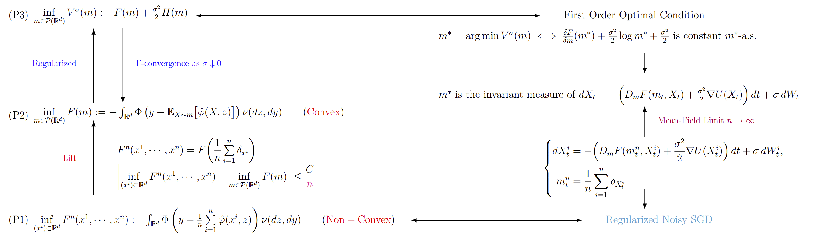Figure 2: Summary of the main analytical framework.

Reference

Hu, Kaitong, et al. “Mean-field Langevin dynamics and energy landscape of neural networks.” Annales de l’Institut Henri Poincare (B) Probabilites et statistiques. Vol. 57. No. 4. Institut Henri Poincaré, 2021.

The cover image of this article was taken at Jungfrau in Switzerland.