Understanding the KKT Conditions

The KKT conditions (Karush–Kuhn–Tucker Conditions) are one of the most important results in optimization, and readers familiar with optimization will certainly not find them unfamiliar. This article will focus on introducing the motivation behind some key concepts introduced in the proof of the KKT conditions (such as the introduction of the active set and the constraint qualification), and will review the complete proof of the KKT conditions.

In this article, we will mainly consider the following nonlinear optimization problem (Nonlinear Optimization Problem, hereinafter abbreviated as NLP):
$$
\begin{aligned}
\min_{x\in \mathbb{R}^n}&\quad f(x),\\\
s.t.&\quad g_i(x) = 0,\quad i=1,\cdots,m_e,\\\
&\quad g_i(x)\ge 0,\quad i=m_e+1,\cdots,m,
\end{aligned}\quad\quad (\text{NLP})
$$
where $f:\mathbb{R}^n\to\mathbb{R}$ and $g_i:\mathbb{R}^n\to\mathbb{R},\ i=1,\cdots,m$ are continuously differentiable.

We denote $\mathcal E = \{1,\cdots,m_e\}$ as the index set consisting of all equality constraints, and $\mathcal I = \{m_e+1,\cdots,m\}$ as the index set consisting of all inequality constraints, and
$$
S = \{x\in\mathbb{R}^n\ |\ g_i(x)=0,\ i\in \mathcal E;\ g_i(x)\ge 0,\ i\in \mathcal I\}
$$
as the feasible set of (NLP). For a given $x\in S$, we call the set of all indices for which equality holds in $S$ the active set of $x$, and denote it by $\mathcal{A}(x)$, that is,
$$
\begin{aligned}
\mathcal{A}(x) &= \mathcal I(x)\cup \mathcal E,\\\
\text{where } \mathcal I(x)&=\{i\in \mathcal I\ |\ g_i(x)=0\}.
\end{aligned}
$$

Before proving the KKT conditions, let us first review the tangent cone, the basic first-order optimality condition, and Farkas’ lemma, which are important foundations for proving the KKT conditions.

Tangent Cone

Definition 1: For $x\in S\subseteq \mathbb{R}^n$, we call

$$
T_S(x) = \left\{d\in\mathbb R^n\ \middle|\ \text{there exist } \{x_k\} \subseteq S,\ x_k\to x,\ \text{and }\{t_k\}\subseteq \mathbb R_+,\ t_k\to 0^+ \text{ such that }\lim_{k\to\infty}\frac{x_k-x}{t_k}=d\right\}
$$

the tangent cone of $S$ at $x$.

Let us first explain the set-theoretic meaning of the definition of the tangent cone: intuitively, for $x\in S\subseteq \mathbb{R}^n$, a direction $d$ in the tangent cone is actually “the opposite direction of those (limiting) directions from which one can keep hitting the point $x$ from within $S$.”

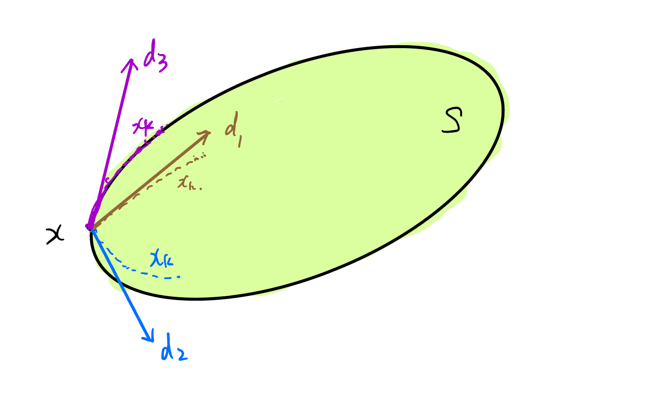
Figure 1: An intuitive understanding of the tangent cone.

Let us look at several examples of tangent cones:

In ①, $S$ is the three edges of a triangle (excluding the interior); in ②, $S$ is the three edges of a triangle including the interior; in ③, $S$ is a circle (excluding the interior); in ④, $S$ is a circle including the interior.

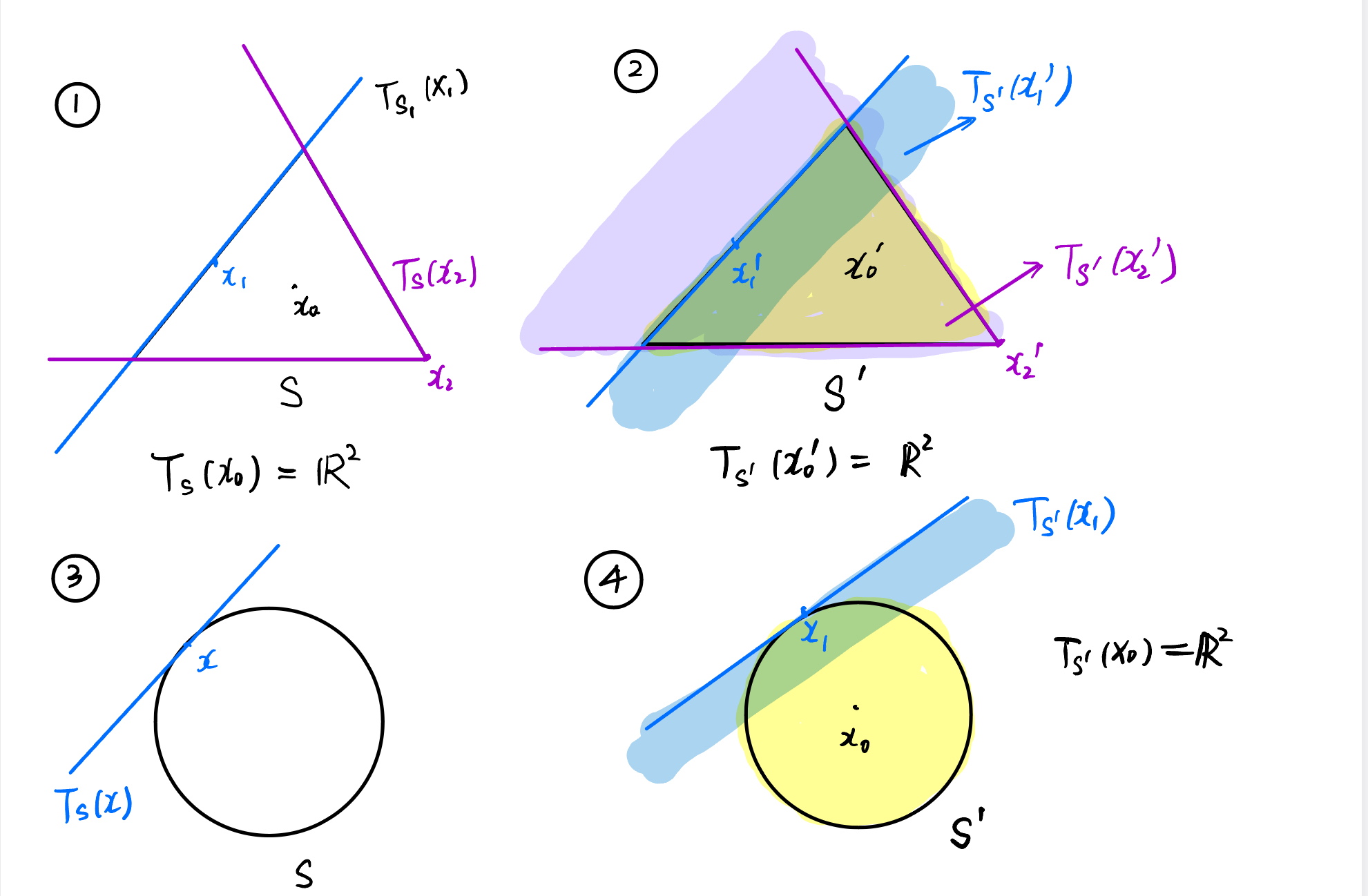
Figure 2: Examples of tangent cones.

Combining these examples, we have a very important observation:

Proposition 1: If $x$ lies in the interior of the set $S$, then necessarily $T_S(x) = \mathbb{R}^n$.

Proof : The proof of this proposition is trivial.

This is a seemingly trivial but in fact very important observation, and this is exactly the motivation for defining the active set (essentially, if $x$ satisfies $g_i(x)>0$ for some $i$, then by the continuity of $g_i$ we know that the set $S_i = \{x|g_i(x)\ge 0\}$ is open, hence $x$ is an interior point of the set $S_i = \{x|g_i(x)\ge 0\}$, and therefore $T_{S_i}(x)=\mathbb{R}^n$; moreover, the intersection of $\mathbb{R}^n$ with any set in $\mathbb{R}^n$ is still that set itself, which is equivalent to not taking the intersection at all).

For the feasible set $S$ of (NLP), we clearly have
$$
S = \bigcap\limits_{i=1}^m S_i,\quad \text{where } S_i = \{x|g_i(x)= 0\},\ i\in\mathcal E;\ S_i = S_i = \{x|g_i(x)\ge 0\},\ i\in \mathcal I
$$
Thus we naturally ask the following question:

Question 1: For $x\in S$, do we have
$$
T_S(x) = \bigcap\limits_{i=1}^m T_{S_i}(x) \ ?
$$

Unfortunately, the answer to Question 1 is negative. A counterexample is as follows:

Consider two circles $S_1$ and $S_2$ tangent at one point $x$ (excluding the interior), and let $S = S_1\cap S_2 = \{x\}$. Then $T_S(x) = \{0\}$, whereas both $T_{S_1}(x)$ and $T_{S_2}(x)$ are the blue-line parts, as shown in the following figure.

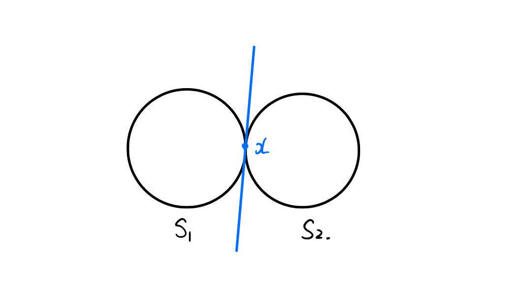
Figure 3: A counterexample to Question 1.

However, we have the following inclusion relation:

Proposition 2: For $x\in S$, we have

$$
T_S(x) \subseteq \bigcap\limits_{i=1}^m T_{S_i}(x).
$$

Proof : For any $d\in T_S(x)$, there exist $\{x_k\}\subseteq S\subseteq S_i,\ i=1,\cdots,m$ and $\{t_k\}\subseteq \mathbb R_+,\ t_k\to 0^+$ such that

$$
\lim_{k\to\infty}\frac{x_k-x}{t_k}=d.
$$

By the definition of $T_{S_i}(x)$, we know that $d\in T_{S_i}(x),\ i=1,\cdots,m$, hence
$$
T_S(x) \subseteq \bigcap\limits_{i=1}^m T_{S_i}(x).
$$

Combining Proposition 1 and Proposition 2, we obtain the following result:

Lemma 1: For $x\in S$, we have
$$
T_S(x) \subseteq \bigcap\limits_{i=1}^m T_{S_i}(x) = \bigcap\limits_{i\in \mathcal{A}(x)} T_{S_i}(x),
$$
where $\mathcal{A}(x)$ is the active set of $x$.

According to Lemma 1, below we only need to consider the active set of $x$.

Now we consider $T_{S_i}(x),\ i\in \mathcal{A}(x)$. From geometric intuition, we can establish a certain connection between $T_{S_i}(x)$ and $\nabla g_i(x)$:

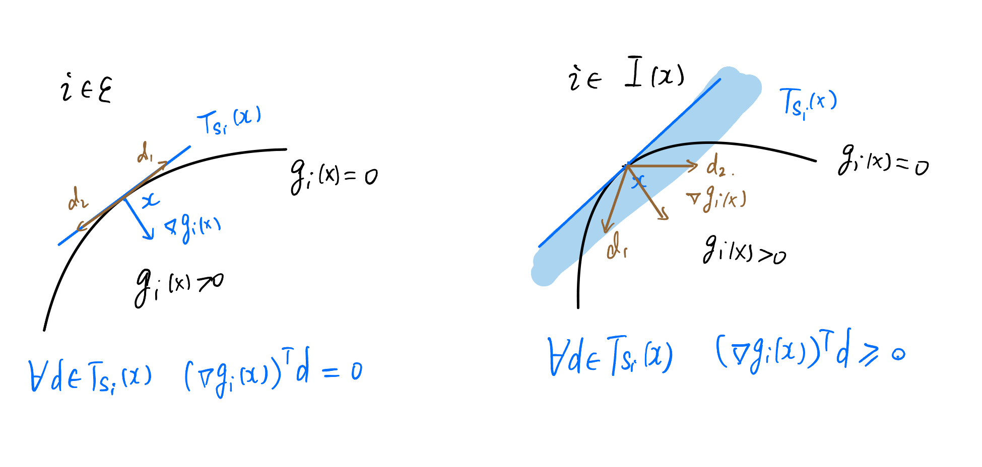
Figure 4: The connection between tangent-cone directions and gradient directions.

Thus we naturally ask the following question:

Question 2: For $i\in \mathcal{A}(x)$, do we necessarily have
$$
T_{S_i}(x) = \{d\in\mathbb{R}^n\ |\ (\nabla g_i(x))^T d=0 \},\quad i\in\mathcal E
$$
$$
T_{S_i}(x) = \{d\in\mathbb{R}^n\ |\ (\nabla g_i(x))^T d\ge 0 \},\quad i\in\mathcal I(x)
$$

Unfortunately, the answer to Question 2 is still negative. In fact, $T_{S_i}(x)$ depends only on the geometric properties of $S_i$, whereas $\nabla g_i$ depends on the expression of $g_i$.

Let us look at the following counterexample:

If $S_i = \{x\in\mathbb{R}\ |\ x^3=0\}$, then $T_{S_i}(0) = \mathbb{R}_+$, but for $g_i(x) = x^3$, the gradient at $0$ is $\nabla g_i(0) = 0$, and hence

$$
\{d\in\mathbb{R}\ |\ (\nabla g_i(x))^T d=0 \}=\mathbb{R},
$$

so the two are not equal. Moreover,

$$
T_{S_i}(x) \subseteq \{d\in\mathbb{R}^n\ |\ (\nabla g_i(x))^T d=0 \},\quad i\in\mathcal E.
$$

Similarly, we have the following inclusion relations:

Lemma 2
$$
T_{S_i}(x) \subseteq \{d\in\mathbb{R}^n\ |\ (\nabla g_i(x))^T d=0 \},\quad i\in\mathcal E
$$
$$
T_{S_i}(x) \subseteq \{d\in\mathbb{R}^n\ |\ (\nabla g_i(x))^T d\ge 0 \},\quad i\in\mathcal I(x)
$$

Proof : First consider the case $i\in\mathcal E$. For any $d\in T_{S_i}(x)$, there exist $\{x_k\}\subseteq S_i$ and $t_k\to 0^+$ such that
$$
\lim_{k\to\infty}\frac{x_k-x}{t_k}=d.
$$
Let
$$
y_k = \frac{x_k-x}{t_k},
$$
then $y_k\to d$. Since $x_k\in S_i$, we have
$$
g_i(x_k) =g_i(x+t_ky_k)=0,\ \forall k.
$$
Consider
$$
\varphi(t)=g_i(x+t y_k).
$$

On the one hand,

$$
\varphi^\prime(0) = \lim_{t\to 0}\frac{g_i(x+ty_k)-g_i(x)}{t} = \lim_{k\to \infty} \frac{g_i(x+t_ky_k)-g_i(x)}{t_k} = 0.\tag{1}
$$

On the other hand,
$$
\varphi^\prime(0) = (\nabla g_i(x))^Ty_k.
$$
Therefore,
$$
(\nabla g_i(x))^Ty_k=0,\ \forall k.
$$
Letting $k\to\infty$, we obtain
$$
(\nabla g_i(x))^Td=0,
$$
that is,
$$
d\in \{d\in\mathbb{R}^n\ |\ (\nabla g_i(x))^T d=0 \}.
$$

For $i\in\mathcal I(x)$, the proof is similar. (In fact, in this case $g_i(x_k) =g_i(x+t_ky_k)\ge 0$, so it suffices to replace (1) by $\ge 0$.)

Summarizing Lemma 1 and Lemma 2, we obtain
$$
T_S(x)\subseteq \{d\in\mathbb{R}^n\ |\ (\nabla g_i(x))^T d=0,\ i\in\mathcal E; \ (\nabla g_i(x))^T d\ge 0,\ i\in\mathcal I(x)\}.
$$
This leads to the definition of the linearized feasible direction cone:

Definition 2 (Linearized Feasible Direction Cone) We call
$$
L(x) = \{d\in\mathbb{R}^n\ |\ (\nabla g_i(x))^T d=0,\ i\in\mathcal E; \ (\nabla g_i(x))^T d\ge 0,\ i\in\mathcal I(x)\}
$$
the linearized feasible direction cone of (NLP).

Summarizing the above, we have the following lemma:

Lemma 3: $T_S(x)\subseteq L(x)$.

Moreover, from the previous counterexample we know that equality does not necessarily hold. In order to make equality hold, we introduce the definition of the constraint qualification:

Definition 3 (Constraint Qualification) A condition under which $T_S(x)= L(x)$ holds is called a constraint qualification.

At this point, we have completed the introduction of the motivation for introducing the active set and the constraint qualification. Next, based on the tangent cone, we give the basic first-order optimality condition.

Basic First-Order Optimality Condition

Theorem 1: Let $x^\star$ be a local minimizer of (NLP), let $f:\mathbb{R}^n\to\mathbb{R}$ and $g_i:\mathbb{R}^n\to\mathbb{R},\ i=1,\cdots,m$ be continuously differentiable, and let $S$ be the feasible set of (NLP). Then for any $d\in T_S(x^\star)$, we have

$$
(\nabla f(x^\star))^Td\ge 0.
$$

Proof : For any $d\in T_S(x^\star)$, there exist $\lbrace x_k\rbrace \subseteq S,\ i=1,\cdots,m$ and $\lbrace t_k\rbrace \subseteq \mathbb R_+,\ t_k\to 0^+$ such that

$$
\lim_{k\to\infty}\frac{x_k-x}{t_k}=d.
$$

Since $x^\star$ is a local minimizer, when $k$ is sufficiently large we have
$$
f(x_k)-f(x^\star)\ge 0.
$$

By the mean value theorem for differentiable functions, there exists $\xi_k$ between $x_k$ and $x$ such that

$$
f(x_k)-f(x^\star) = (\nabla f(\xi_k))^T(x_k-x^\star).
$$

Hence, for sufficiently large $k$,

$$
\frac{f(x_k)-f(x^\star)}{t_k} =(\nabla f(\xi_k))^T\frac{x_k-x^\star}{t_k}\ge 0.
$$

Letting $k\to\infty$, by the continuity of $\nabla f$ we obtain

$$
(\nabla f(x^\star))^Td\ge 0.
$$

According to the constraint qualification, we know that $L(x^\star) = T_S(x^\star)$, and therefore for any $d\in L(x^\star)$, we must have $d\in T_S(x^\star)$, that is,

$$
\left.
\begin{matrix}
i\in\mathcal E, \ (\nabla g_i(x^\star))^Td=0\\\
i\in\mathcal I(x^\star), \ (\nabla g_i(x^\star))^Td\ge 0
\end{matrix}
\right\}\Longrightarrow (\nabla f(x^\star))^Td\ge 0.
$$

In order to further obtain the KKT conditions, we need Farkas’ lemma.

Theorem 2 (Farkas’ Lemma) For $A\in \mathbb{R}^{m\times n}$ and $b\in \mathbb{R}^n$, the following statements are equivalent:

(1) For any $d\in \mathbb{R}^n$, if $Ad\ge 0$, then $b^Td\ge 0$.

(2) There exists $\lambda\in \mathbb{R}^m,\ \lambda\ge 0$ such that $A^T\lambda = b$.

Farkas’ lemma requires the separating hyperplane theorem for convex sets. Since its proof would depart from the main line, we omit it here. Interested readers may consult the relevant literature by themselves.

Here we only present the geometric meaning of Farkas’ lemma.

Let $A^T = [a_1,a_2,\cdots,a_m]$. Then Farkas’ lemma states that $b$ lies in the convex cone generated by the vectors $a_1,\cdots,a_m$ if and only if whenever $d$ forms an acute angle with the vectors $a_1,\cdots,a_m$, then $d$ also forms an acute angle with $b$, as shown in the following figure:

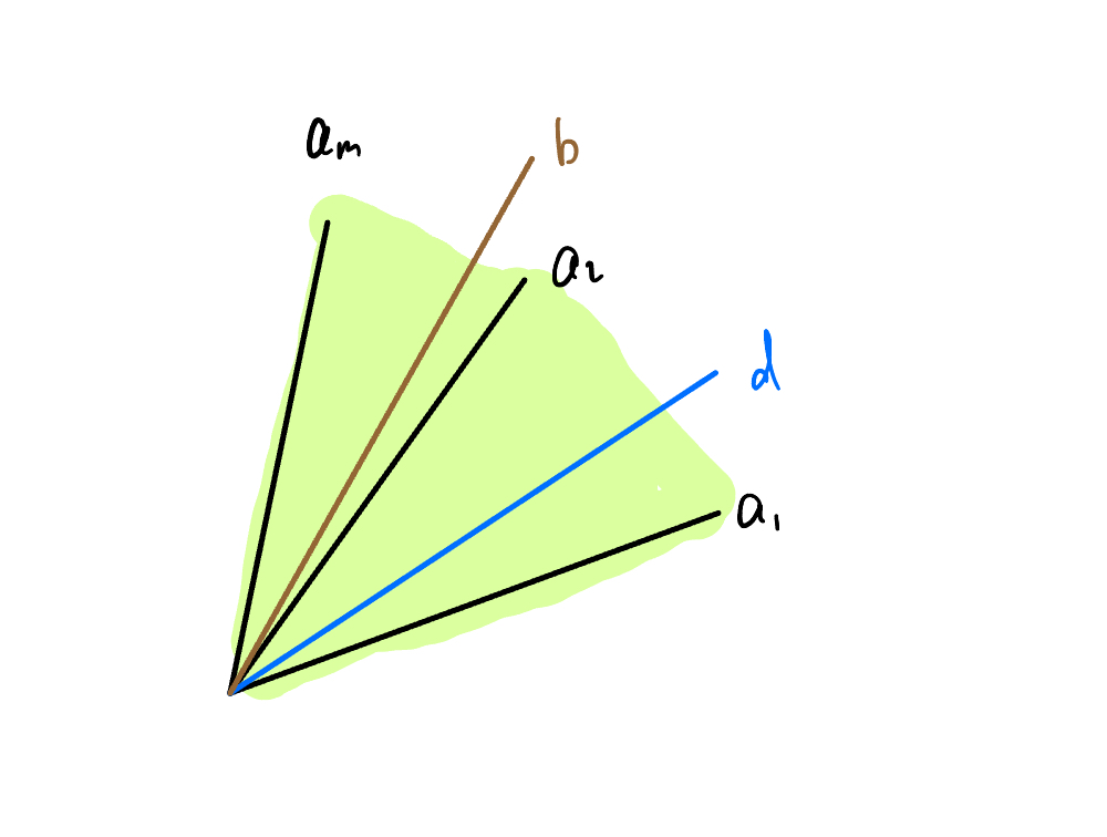
Figure 5: Geometric interpretation of Farkas' lemma.

Based on the above analysis, we now give the KKT conditions.

KKT Conditions

Theorem 3 (KKT Conditions) Let $x^\star$ be a local minimizer of (NLP), let $f:\mathbb{R}^n\to\mathbb{R}$ and $g_i:\mathbb{R}^n\to\mathbb{R},\ i=1,\cdots,m$ be continuously differentiable, let $S$ be the feasible set of (NLP), and suppose that $T_S(x^\star) = L(x^\star)$ holds. Then there exists $\lambda^\star\in \mathbb{R}^m$ such that the following hold:

• (Stationarity condition): $\nabla f(x^\star)-\sum\limits_{i=1}^m \lambda_i^\star\nabla g_i(x^\star) = 0$.
• (Primal feasibility condition): $g_i(x^\star) = 0,\ \forall i\in \mathcal E$ and $g_i(x^\star) \ge 0,\ \forall i\in \mathcal I$.
• (Dual feasibility condition): $\lambda_i^\star\ge 0,\ \forall i\in \mathcal I$.
• (Complementary slackness condition): $\lambda_i^\star g_i(x^\star)=0,\ \forall i\in\mathcal I$.

Proof : Since $x^\star$ is a local minimizer of (NLP) and $T_S(x^\star) = L(x^\star)$, we have

$$
\left.
\begin{matrix}
i\in\mathcal E, \ (\nabla g_i(x^\star))^Td=0\\\
i\in\mathcal I(x^\star), \ (\nabla g_i(x^\star))^Td\ge 0
\end{matrix}
\right\}\Longrightarrow (\nabla f(x^\star))^Td\ge 0.\quad (2)
$$

Let

$$
A = \begin{pmatrix}
(\nabla g_i(x^\star))^T,\quad(i\in \mathcal E)\\\
-(\nabla g_i(x^\star))^T,\quad(i\in \mathcal E)\\\
(\nabla g_i(x^\star))^T,\quad(i\in \mathcal I(x^\star))
\end{pmatrix}.
$$

From (2), we know that whenever $Ad\ge 0$, we have

$$
(\nabla f(x^\star))^Td\ge 0.
$$

Therefore, by Farkas’ lemma, there exists

$$
\begin{pmatrix}
\lambda\\\
\mu_+\\\
\mu_-
\end{pmatrix}\ge 0
$$

such that

$$
A^T\begin{pmatrix}
\lambda\\\
\mu_+\\\
\mu_-
\end{pmatrix} =\nabla f(x^\star).
$$

Define

$$
\lambda_i^\star = \lambda_i,\quad \forall i\in \mathcal I(x^\star)
$$

$$
\lambda_i^\star = 0,\quad \forall i\in \mathcal I\backslash\mathcal I(x^\star)
$$

$$
\lambda_i^\star = \mu_+-\mu_-,\quad \forall i\in \mathcal E.
$$

It is not difficult for the reader to verify that the KKT conditions hold.

The cover image of this article was taken in Colmar, France.