Introduction to Flow Matching

In generative modeling, we are given a collection of training samples $\{x_i\}_{i=1}^N$ and wish to generate new samples from the underlying target distribution $\pi$. There are already many established approaches to this problem, including likelihood-based methods, implicit generative models such as GANs, and score-based diffusion models. More recently, the flow matching framework has emerged as another powerful paradigm. In what follows, we introduce the basic ideas of flow matching and explain how works.

Background

For a particle initially at position $x_0 \in \mathbb{R}^d$ and a (Lipschitz continuous) velocity field $\{v_t\}$, there exists a unique trajectory $\{x_t\}$ described by

$$
\begin{cases}
\begin{split}
\dfrac{d x_t}{dt} &= v_t(x_t),\quad t\in [0,1]\\\
x_0&=x_0
\end{split}
\end{cases}.\tag{Flow-ODE}
$$
The flow $\Phi$ collects the trajectories corresponding to different initial positions $x_0$ and is defined by

$$
\begin{split}
\Phi: [0,1]\times \mathbb{R}^d&\to \mathbb{R}^d\\\
(t,x_0)&\mapsto \Phi(t,x_0)=x_t,
\end{split}
$$
where $x_t$ denotes the solution of (Flow-ODE) at time $t$.

If the flow mapping $\Phi$ is known, then for any initial position $x_0 \in \mathbb{R}^d$ we can obtain the terminal position $x_1$ via $x_1 = \Phi(1,x_0)$. To determine the flow mapping $\Phi$, it suffices to know the velocity field $\{v_t\}_{t \in [0,1]}$ and to solve the ordinary differential equation (Flow-ODE).

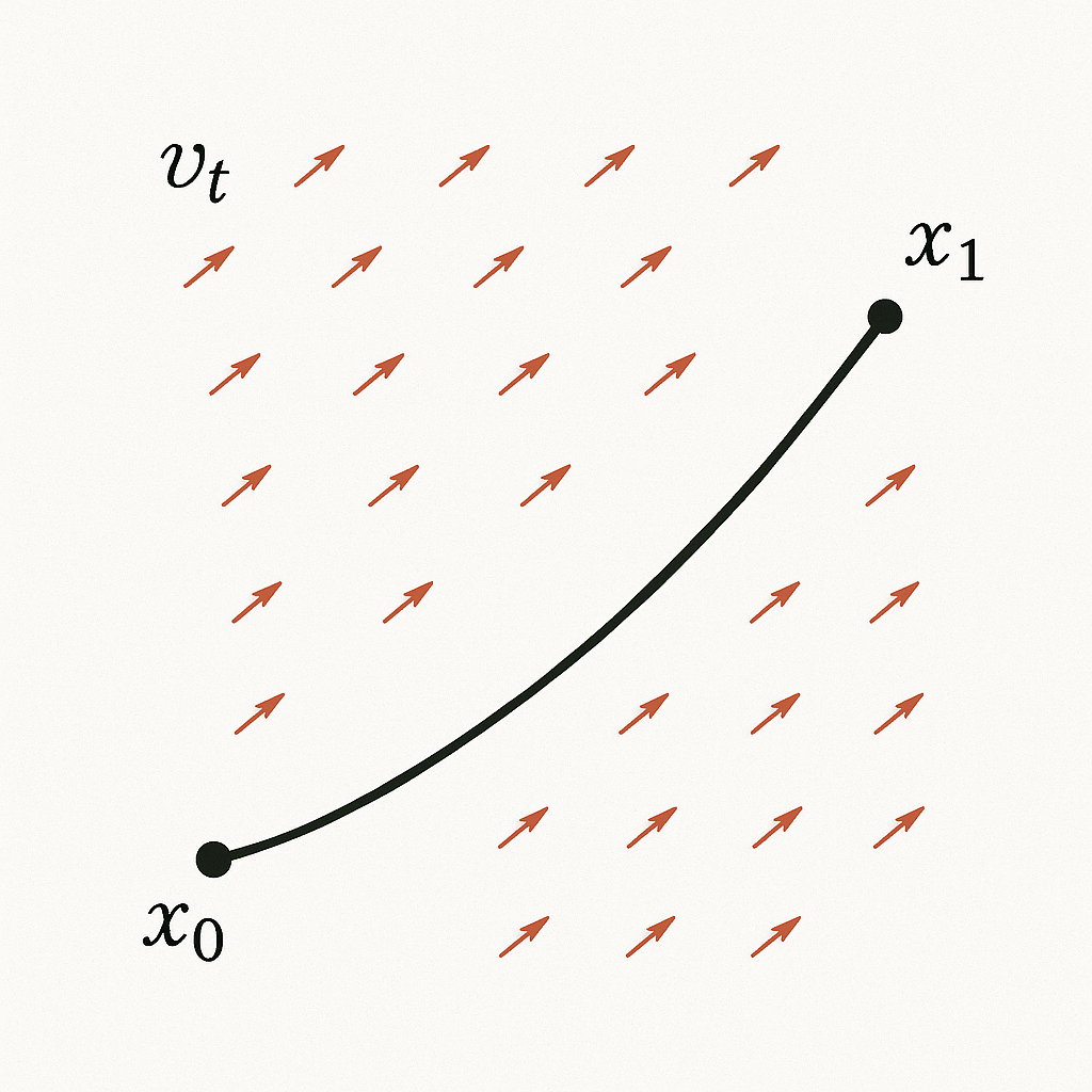
Figure 1: A particle moves from $x_0$ to $x_1$ along the velocity field $v_t$.

In general, we aim to use the flow mapping $\Phi$ to transport the initial distribution $\mu_0$ to the target distribution $\pi$.

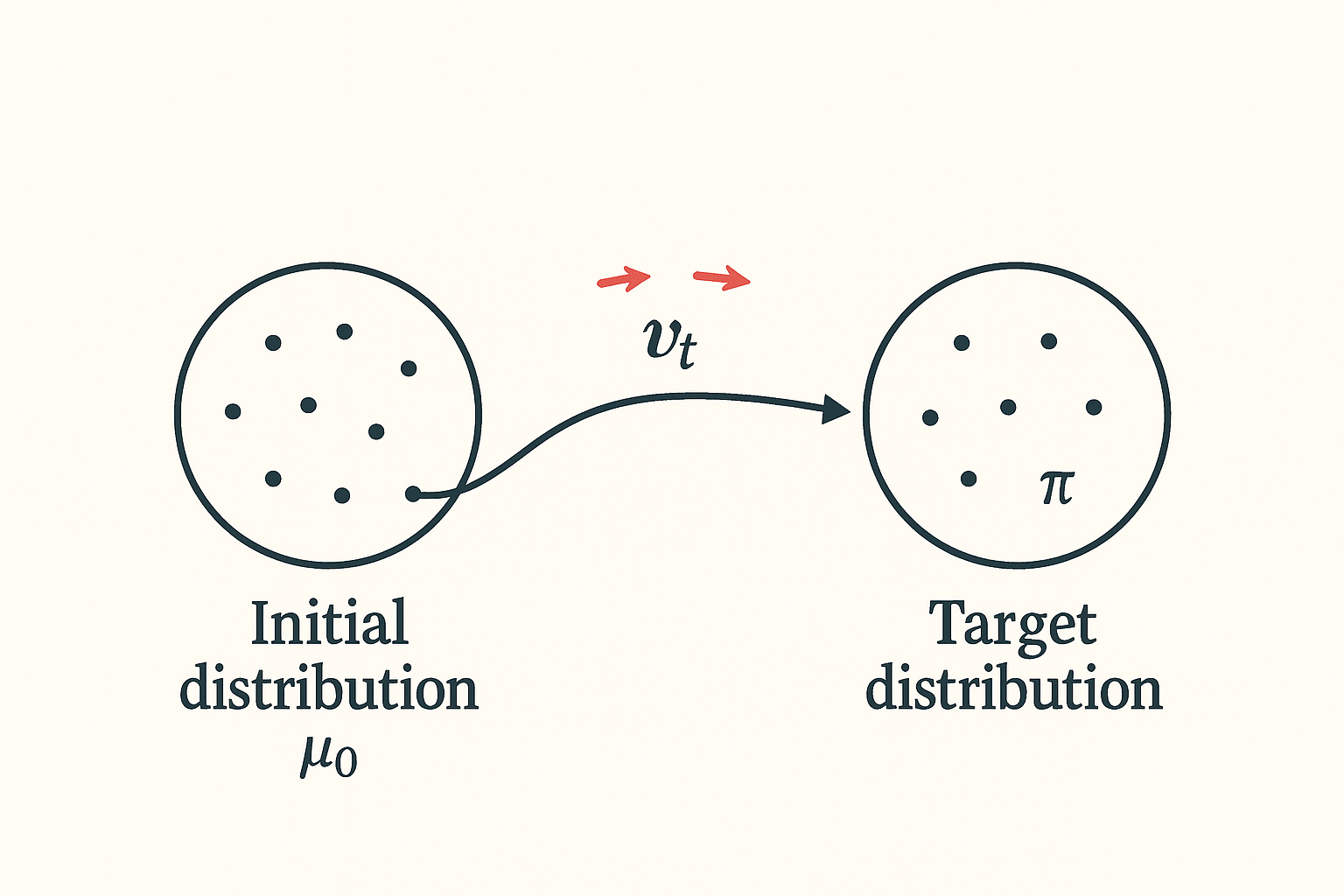
Figure 2: Transport the initial distribution $\mu_0$ to the target distribution $\pi$ by the flow mapping $\Phi$ (or the corresponding vector field $v_t$).

Let $\{X_t\}$ be a stochastic process with $\operatorname{Law}(X_t)=\mu_t$ such that
$$
\begin{cases}
\begin{split}
\dfrac{d X_t}{dt} &= v_t(X_t),\ a.e. \\\
X_0&\sim \mu_0
\end{split}
\end{cases},\quad t\in [0,1]
$$
Then we know $(\mu_t,v_t)$ must satisfies the following continuity equation
$$
\partial_t \mu_t +\nabla\cdot (\mu_tv_t) = 0,
$$
which means for all $\varphi\in C_c^{\infty}((0,1)\times \mathbb{R}^d)$, we have
$$
\int_{0}^{1}\int_{\mathbb{R}^d}\left[\dfrac{\partial}{\partial t}\varphi(t,y)+\langle v_t(y), \nabla\varphi(t,y)\rangle\right]\mu_t(dy)dt=0.\tag{CE}
$$
If $\mu_t$ has density $\rho_t$ with respect to Lebesgue measure on $\mathbb{R}^d$, continuity equation can be written as
$$
\partial_t \rho_t +\nabla\cdot (\rho_tv_t) = 0.
$$

Note: The ODE formulation
$$
\begin{cases}
\begin{split}
\dfrac{d X_t}{dt} &= v_t(X_t),\ \text{a.e.} \\\
X_0 &\sim \mu_0
\end{split}
\end{cases}\qquad t\in [0,1]
$$
is the Lagrangian (particle) viewpoint, while the continuity equation
$$
\partial_t \mu_t + \nabla\cdot(\mu_t v_t) = 0
$$
is the Eulerian (distribution) viewpoint. One can show that the Lagrangian formulation implies the Eulerian one. Conversely, under suitable assumptions, if the continuity equation holds, then there exists a stochastic process $(X_t)_{t\in[0,1]}$ solving the ODE above. This result is often referred to as the superposition principle (see [1] for a reference).

Hence, once we have learned a “good” flow map $\Phi$, we can sample $X_0$ from the initial distribution $\mu_0$ (for instance, a Gaussian $N(0, I_d)$), and then obtain
$$
\operatorname{Law}(X_1) =\operatorname{Law}(\Phi(1, X_0)) =\mu_1 \approx \pi.
$$
The central question is therefore: how can we learn such a “good” flow map $\Phi$, or equivalently, how can we design the vector field $\{v_t\}$ using only the training data $\{x_i\}_{i=1}^N \stackrel{\text{i.i.d.}}{\sim} \pi$?

Flow Matching

The main idea of flow matching is to approximate the target vector field $v_t$ by a neural network $u_t^{(\theta)}$. The neural network is trained by minimizing a suitable discrepancy between $u_t^{(\theta)}$ and an explicitly known conditional vector field $v_t^x$. To make this precise, we first introduce the conditional probability paths $\mu_t^x$ and the corresponding conditional vector fields $v_t^x$, and then explain how they relate to the marginal probability path $\mu_t$ and the marginal vector field $v_t$ that we ultimately wish to learn.

Conditional Probability Path and Conditional Vector Field

Definition 1. The conditional probability path is a path of Markov kernel denoted by $\mu_t^x$ satisfying:

(1) For all $t\in [0,1]$ and $A\in \mathcal{B}(\mathbb{R}^d)$, the mapping $x\mapsto \mu_t^x(A)$ is $\mathcal{B}(\mathbb{R}^d)$-measurable;

(2) For all $t\in [0,1]$ and $x\in \mathbb{R}^d$, $\mu_t^x(\cdot)$ is a probability measure on $\mathbb{R}^d$;

(3) For all $x\in \mathbb{R}^d$, $\mu_0^x\equiv \mu_0$ and $\mu_1^x=\delta_x$.

Note: Property (3) above is used to ensure that the marginal probability path
$$
\mu_t(A) := \int_{\mathbb{R}^d} \mu_t^x(A)\ \pi(dx), \quad \forall A \in \mathcal{B}(\mathbb{R}^d),
$$
satisfies $\mu_0 = \mu_0$ (our prescribed initial distribution) and
$$
\mu_1(A) = \int_{\mathbb{R}^d} \delta_x(A)\ \pi(dx) = \int_A \pi(dx) = \pi(A), \quad \forall A \in \mathcal{B}(\mathbb{R}^d),
$$
which implies that $\mu_1 = \pi$. Hence $\mu_t$ is a probability path interpolating between the initial distribution $\mu_0$ and the target distribution $\pi$, which is exactly what we want.

In practice, one may choose a sufficiently small $\sigma_{\min} > 0$ and set $\mu_1^x = N(x, \sigma_{\min}^2)$, so that in the end $\mu_1 \approx \pi$.

Construction of Conditional Probability Path

There are many ways to construct a conditional probability path $\mu_t^x$ satisfying the conditions in Definition 1. Here, we adopt a simple conditional Gaussian path
$$
\mu_t^x = N(m_t^x,(\sigma_t^x)^2I_d),
$$
where
$$
m_t^x = tx\quad \text{and}\quad (\sigma_t^x)^2 = (1-t)^2\sigma_0^2+\sigma_{\min}^2,
$$
with $\sigma_0^2=1-\sigma_{\min}^2$. It is easy to see that
$$
\mu_0^x = N(0,I_d)\quad \text{and}\quad \mu_1^x = N(x,\sigma_{\min}^2I_d)\approx \delta_x.
$$
Naturally, we hope our trajectory is
$$
Y_t^x = m_t^x+\sigma_t^x Z,
$$
where $Z\sim N(0,I_d)$ and we have $\operatorname{Law}(Y_t^x)=\mu_t^x$. By differentiating $Y_t^x$ with respect to $t$, we obtain
$$
\begin{aligned}
\dfrac{d}{dt}Y_t^x &= \dot m_t^x+\dot \sigma_t^x Z\\\
&=\dot m_t^x+\dfrac{\dot \sigma_t^x}{\sigma_t^x} (Y_t^x-m_t^x),
\end{aligned}
$$
where $\dot m_t^x = \dfrac{d}{dt} m_t^x$ and $\dot \sigma_t^x = \dfrac{d}{dt} \sigma_t^x$. Hence, we can choose the conditional vector field
$$
v_t^x(y):= \dot m_t^x+\dfrac{\dot \sigma_t^x}{\sigma_t^x} (y-m_t^x).
$$
Then we have
$$
\begin{cases}
\dfrac{d}{dt}Y_t^x = v_t^x(Y_t^x),\ \operatorname{Law}(Y_t^x)=\mu_t^x\\\
Y_0^x\sim \mu_0^x
\end{cases},\quad t\in [0,1].
$$
Therefore, $(\mu_t^x, v_t^x)$ satisfies the continuity equation: for all $\varphi\in C_c^{\infty}((0,1)\times \mathbb{R}^d)$, we have
$$
\int_{0}^{1}\int_{\mathbb{R}^d}\left[\dfrac{\partial}{\partial t}\varphi(t,y)+\langle v_t^x(y), \nabla\varphi(t,y)\rangle\right]\mu_t^x(dy)dt=0.\tag{CE-conditional}
$$

Summary

We construct the conditional probability path
$$
\mu_t^x = N(m_t^x,(\sigma_t^x)^2I_d),
$$
where
$$
m_t^x = tx\quad \text{and}\quad (\sigma_t^x)^2 = (1-t)^2\sigma_0^2+\sigma_{\min}^2,
$$
with $\sigma_0^2=1-\sigma_{\min}^2$ and it satisfies
$$
\mu_0^x = N(0,I_d)\quad \text{and}\quad \mu_1^x = N(x,\sigma_{\min}^2I_d)\approx \delta_x.
$$
Then we construct the conditional vector field
$$
v_t^x(y):= \dot m_t^x+\dfrac{\dot \sigma_t^x}{\sigma_t^x} (y-m_t^x).
$$
And then $(\mu_t^x, v_t^x)$ satisfies the continuity equation: for all $\varphi\in C_c^{\infty}((0,1)\times \mathbb{R}^d)$, we have
$$
\int_{0}^{1}\int_{\mathbb{R}^d}\left[\dfrac{\partial}{\partial t}\varphi(t,y)+\langle v_t^x(y), \nabla\varphi(t,y)\rangle\right]\mu_t^x(dy)dt=0.\tag{CE-conditional}
$$

Marginal Probability Path and Marginal Vector Field

We define the marginal probability path $\mu_t$ by
$$
\mu_t(A) := \int_{\mathbb{R}^d} \mu_t^x(A)\ \pi(dx), \quad \forall A \in \mathcal{B}(\mathbb{R}^d).
$$
We have $\mu_t$ start at our initial distribution $\mu_0$ and end by
$$
\mu_1\approx \pi.
$$
What’s more, we have the following lemma.

Lemma 1. For $\pi-$a.e. $x$, we have $\mu_t^x\ll \mu_t$.

Proof : If $\mu_t(A)=0$, then
$$
\int_{\mathbb{R}^d} \mu_t^x(A)\ \pi(dx)=0.
$$
Since $\mu_t^x(A)\ge 0$, we have for $\pi-$a.e. $x$, $\mu_t^x(A)=0$. Hence, for $\pi-$a.e. $x$, we have $\mu_t^x\ll \mu_t$.

By Lemma 1, for $\pi-$a.e. $x$, the Radon-Nikodym derivative
$$
\dfrac{d\mu_t^x}{d\mu_t}
$$
exists. Then we can define the marginal vector field as
$$
v_t(y):= \int_{\mathbb{R}^d} v_t^x(y) \dfrac{d\mu_t^x}{d\mu_t}(y)\pi(dx).
$$
Note: To some extent, $v_t$ is a weighted average of $v_t^x$.

Theorem 2. $(\mu_t, v_t)$ satisfies the continuity equation.

Proof : For all $\varphi\in C_c^{\infty}((0,1)\times \mathbb{R}^d)$, we need to show that
$$
I=\int_{0}^{1}\int_{\mathbb{R}^d}\left[\dfrac{\partial}{\partial t}\varphi(t,y)+\langle v_t(y), \nabla\varphi(t,y)\rangle\right]\mu_t(dy)dt=0.
$$
In fact, $I=I_1+I_2$, where
$$
\begin{aligned}
I_1&=\int_{0}^{1}\int_{\mathbb{R}^d}\dfrac{\partial}{\partial t}\varphi(t,y)\mu_t(dy)dt\\\
I_2&=\int_{0}^{1}\int_{\mathbb{R}^d}\langle v_t(y), \nabla\varphi(t,y)\rangle\mu_t(dy)dt.
\end{aligned}
$$
By using
$$
\mu_t(dy) =\int_{\mathbb{R}^d} \mu_t^x(dy)\ \pi(dx)
$$
and
$$
v_t(y):= \int_{\mathbb{R}^d} v_t^x(y) \dfrac{d\mu_t^x}{d\mu_t}(y)\ \pi(dx),
$$
we have
$$
\begin{aligned}
I_1&=\int_{0}^{1}\int_{\mathbb{R}^d}\dfrac{\partial}{\partial t}\varphi(t,y)\ \mu_t(dy)\ dt\\\
&=\int_{0}^{1}\int_{\mathbb{R}^d}\int_{\mathbb{R}^d}\dfrac{\partial}{\partial t}\varphi(t,y)\ \mu_t^x(dy)\ \pi(dx)\ dt\\\
&\xlongequal{\text{Fubini}}\int_{\mathbb{R}^d}\int_{0}^{1}\int_{\mathbb{R}^d}\dfrac{\partial}{\partial t}\varphi(t,y)\ \mu_t^x(dy)\ dt\ \pi(dx)
\end{aligned}
$$
and
$$
\begin{aligned}
I_2&=\int_{0}^{1}\int_{\mathbb{R}^d}\langle v_t(y), \nabla\varphi(t,y)\rangle\ \mu_t(dy)\ dt\\\
&=\int_{0}^{1}\int_{\mathbb{R}^d}\int_{\mathbb{R}^d}\langle v_t^x(y), \nabla\varphi(t,y)\rangle\ \dfrac{d\mu_t^x}{d\mu_t}(y)\ \pi(dx)\ \mu_t(dy)\ dt\\\
&\xlongequal{\text{Fubini}}\int_{\mathbb{R}^d}\int_{0}^{1}\int_{\mathbb{R}^d}\langle v_t^x(y), \nabla\varphi(t,y)\rangle\ \dfrac{d\mu_t^x}{d\mu_t}(y)\ \mu_t(dy)\ dt \ \pi(dx)\\\
&\xlongequal{\text{Chain Rule}}\int_{\mathbb{R}^d}\int_{0}^{1}\int_{\mathbb{R}^d}\langle v_t^x(y), \nabla\varphi(t,y)\rangle\ \mu_t^x(dy)\ dt \ \pi(dx).
\end{aligned}
$$
Hence by $(\mu_t^x, v_t^x)$ satisfies the continuity equation, namely
$$
\int_{0}^{1}\int_{\mathbb{R}^d}\left[\dfrac{\partial}{\partial t}\varphi(t,y)+\langle v_t^x(y), \nabla\varphi(t,y)\rangle\right]\mu_t^x(dy)dt=0
$$
we get
$$
I=I_1+I_2 =\int_{\mathbb{R}^d}\int_{0}^{1}\int_{\mathbb{R}^d}\left[\dfrac{\partial}{\partial t}\varphi(t,y)+\langle v_t^x(y), \nabla\varphi(t,y)\rangle\right]\ \mu_t^x(dy)\ dt\ \pi(dx)=0,
$$
which means $(\mu_t, v_t)$ satisfies the continuity equation.

By Theorem 2, there exists a stochastic process $X_t$ with $\operatorname{Law}(X_t)=\mu_t$ such that
$$
\begin{cases}
\begin{split}
\dfrac{d X_t}{dt} &= v_t(X_t),\ a.e. \\\
X_0&\sim \mu_0
\end{split}
\end{cases},\quad t\in [0,1]
$$
And $\mu_t$ start at our initial distribution $\mu_0$ and end by
$$
\mu_1\approx \pi.
$$

Summary

We construct the marginal probability path and marginal vector field by
$$
\begin{aligned}
\mu_t(A) &:= \int_{\mathbb{R}^d} \mu_t^x(A)\ \pi(dx), \quad \forall A \in \mathcal{B}(\mathbb{R}^d).\\\
v_t(y)&:= \int_{\mathbb{R}^d} v_t^x(y) \dfrac{d\mu_t^x}{d\mu_t}(y)\pi(dx).
\end{aligned}
$$
We have $(\mu_t, v_t)$ satisfies the continuity equation, which means there exists a stochastic process $X_t$ with $\operatorname{Law}(X_t)=\mu_t$ such that
$$
\begin{cases}
\begin{split}
\dfrac{d X_t}{dt} &= v_t(X_t),\ a.e. \\\
X_0&\sim \mu_0
\end{split}
\end{cases},\quad t\in [0,1].
$$
And $\mu_t$ start at our initial distribution $\mu_0$ and end by
$$
\mu_1\approx \pi.
$$

Now we can answer the question about how to train the neural network $u_t^{(\theta)}$.

Training

Theorem 3. Define the marginal loss $L(\theta)$ and conditional loss $J(\theta)$ by
$$
\begin{aligned}
L(\theta)&:= \int_{0}^{1}\int_{\mathbb{R}^d}|v_t(y)-u_t^{(\theta)}(y)|^2\ \mu_t(dy)\ dt\\\
J(\theta)&:= \int_{0}^{1}\int_{\mathbb{R}^d}\int_{\mathbb{R}^d}|v_t^x(y)-u_t^{(\theta)}(y)|^2\ \mu_t^x(dy)\ \pi(dx)\ dt
\end{aligned}
$$
We have
$$
L(\theta) = J(\theta)+C,
$$
where $C$ is a constant independent of $\theta$. Hence,
$$
\arg\min_{\theta} L(\theta)=\arg\min_{\theta} J(\theta).
$$
Proof : Expand $L(\theta),\ J(\theta)$ as
$$
L(\theta) = A_1-2B_1+C_1,
$$
where
$$
A_1 = \int_{0}^{1}\int_{\mathbb{R}^d}|v_t(y)|^2\ \mu_t(dy)\ dt,\ B_1= \int_{0}^{1}\int_{\mathbb{R}^d}\langle v_t(y), u_t^{(\theta)}(y)\rangle\ \mu_t(dy)\ dt,\ C_1= \int_{0}^{1}\int_{\mathbb{R}^d}|u_t^{(\theta)}|^2\ \mu_t(dy)\ dt
$$
and
$$
J(\theta) = A_2-2B_2+C_2,
$$
where
$$
A_2= \int_{0}^{1}\int_{\mathbb{R}^d}\int_{\mathbb{R}^d}|v_t^x(y)|^2\ \mu_t^x(dy)\ \pi(dx)\ dt,\ B_2=\int_{0}^{1}\int_{\mathbb{R}^d}\int_{\mathbb{R}^d}\langle v_t^x(y), u_t^{(\theta)}(y)\rangle\ \mu_t^x(dy)\ \pi(dx)\ dt,\ C_2= \int_{0}^{1}\int_{\mathbb{R}^d}\int_{\mathbb{R}^d}|u_t^{(\theta)}|^2\ \mu_t^x(dy)\ \pi(dx)\ dt.
$$
By using
$$
\mu_t(dy) =\int_{\mathbb{R}^d} \mu_t^x(dy)\ \pi(dx)
$$
and
$$
v_t(y):= \int_{\mathbb{R}^d} v_t^x(y) \dfrac{d\mu_t^x}{d\mu_t}(y)\ \pi(dx),
$$
we have
$$
\begin{aligned}
C_1 &= \int_{0}^{1}\int_{\mathbb{R}^d}|u_t^{(\theta)}|^2\ \mu_t(dy)\ dt\\\
&= \int_{0}^{1}\int_{\mathbb{R}^d}\int_{\mathbb{R}^d}|u_t^{(\theta)}|^2\ \mu_t^x(dy)\ \pi(dx)\ dt\\\
&=C_2
\end{aligned}
$$
and
$$
\begin{aligned}
B_1&= \int_{0}^{1}\int_{\mathbb{R}^d}\langle v_t(y), u_t^{(\theta)}(y)\rangle\ \mu_t(dy)\ dt\\\
&=\int_{0}^{1}\int_{\mathbb{R}^d}\int_{\mathbb{R}^d}\langle v_t^x(y), u_t^{(\theta)}(y)\rangle\ \dfrac{d\mu_t^x}{d\mu_t}(y)\ \pi(dx)\ \mu_t(dy)\ dt\\\
&\xlongequal{\text{Fubini}}\int_{0}^{1}\int_{\mathbb{R}^d}\int_{\mathbb{R}^d}\langle v_t^x(y), u_t^{(\theta)}(y)\rangle\ \dfrac{d\mu_t^x}{d\mu_t}(y)\ \mu_t(dy)\ \pi(dx)\ dt\\\
&\xlongequal{\text{Chain Rule}} \int_{0}^{1}\int_{\mathbb{R}^d}\int_{\mathbb{R}^d}\langle v_t^x(y), u_t^{(\theta)}(y)\rangle\ \mu_t^x(dy)\ \pi(dx)\ dt\\\
&=B_2.
\end{aligned}
$$
Since $A_1$ and $A_2$ are independent of $\theta$, the desired result follows directly.

By Theorem 3, we can

• sample $\{t_k\}_{k=1}^K\sim U[0,1]$;
• draw from training dataset $\{x_i\}_{i=1}^N$;
• for all $(t_k, x_i)$, draw $M$ samples $\{y_m^{(t_k,x_i)}\}_{m=1}^M\sim \mu_t^x=N(m_t^x,(\sigma_t^x)^xI_d)$.

And then train our neural network by
$$
\min_\theta\quad\dfrac{1}{KNM}\sum_{k=1}^K\sum_{i=1}^N\sum_{m=1}^M |v_{t_k}^{x_i}(y_m^{(t_k,x_i)})-u_{t_k}^{(\theta)}(y_m^{(t_k,x_i)})|^2.
$$

Summary

Our goal is to sample from the target distribution $\pi$. To this end, we first draw samples (for example $x_0$) from an initial distribution $\mu_0=N(0,I_d)$ and then apply a trained vector field $u_t^{(\theta)}$, so that at the terminal time we obtain samples (corresponding $x_1$) distributed (approximately) according to $\pi$ by solving the following ODE
$$
\begin{cases}
\begin{split}
\dfrac{d x_t}{dt} &= u_t^{(\theta)}(x_t),\quad t\in [0,1]\\\
x_0&=x_0
\end{split}
\end{cases}
$$
by numerical method such as the Euler method or the Runge-Kutta method. The way to training the vector field $u_t^{(\theta)}$​ is by
$$
\min_\theta\quad\dfrac{1}{KNM}\sum_{k=1}^K\sum_{i=1}^N\sum_{m=1}^M |v_{t_k}^{x_i}(y_m^{(t_k,x_i)})-u_{t_k}^{(\theta)}(y_m^{(t_k,x_i)})|^2,
$$
where $t_k\sim U[0,1], k=1,\cdots,K$ and $x_i,\ i=1,\cdots,N$ draw from training dataset,
$$
\{y_m^{(t_k,x_i)}\}_{m=1}^M\sim \mu_t^x=N(m_t^x,(\sigma_t^x)^xI_d)
$$

and
$$
v_{t}^{x}(y):= \dot m_t^x+\dfrac{\dot \sigma_t^x}{\sigma_t^x} (y-m_t^x)
$$
with $m_t^x = tx\quad \text{and}\quad (\sigma_t^x)^2 = (1-t)^2\sigma_0^2+\sigma_{\min}^2$ , $\sigma_0^2=1-\sigma_{\min}^2$.

There are mainly three types of errors

• (terminal error) since $\mu_1^x=N(x,\sigma_{\min}^2I_d)\approx \delta_x$, there is an error between $\mu_1$ and target distribution $\pi$, but we can control this error by choosing $\sigma_\min$ sufficiently small.
• (discretization error) there is an error when solving the ODE above numerically, but we can control this error by choosing step size $h$ sufficiently small.
• (flow matching error) there is an error between $u_t^{(\theta)}$ and true vector field $v_t$, but we can assume the neural network can be trained well enough to make this error small enough.

In conclusion: Sampling is as easy as learning the vector field!

Reference

[1] Ambrosio, Luigi, Nicola Gigli, and Giuseppe Savaré. Gradient flows: in metric spaces and in the space of probability measures. Basel: Birkhäuser Basel, 2005.

[2] Lipman, Yaron, et al. “Flow matching for generative modeling.” arXiv preprint arXiv:2210.02747 (2022).

[3] Kerrigan, Gavin, Giosue Migliorini, and Padhraic Smyth. “Functional flow matching.” arXiv preprint arXiv:2305.17209 (2023).

The cover image of this article was taken on the Great Ocean Road, Australia.