<?xml version="1.0" encoding="utf-8"?>
<feed xmlns="http://www.w3.org/2005/Atom">
  <author>
    <name>Handstein Wang</name>
  </author>
  <generator uri="https://hexo.io/">Hexo</generator>
  <id>https://handsteinwang.github.io/</id>
  <link href="https://handsteinwang.github.io/" rel="alternate"/>
  <link href="https://handsteinwang.github.io/atom.xml" rel="self"/>
  <rights>All rights reserved 2026, Handstein Wang</rights>
  <title>Handstein Wang</title>
  <updated>2026-04-15T16:00:00.000Z</updated>
  <entry>
    <author>
      <name>Handstein Wang</name>
    </author>
    <category term="Gradient Flows" scheme="https://handsteinwang.github.io/categories/Gradient-Flows/"/>
    <category term="Gradient Flows" scheme="https://handsteinwang.github.io/tags/Gradient-Flows/"/>
    <content>
      <![CDATA[<p>In this article, we will introduce the gradient flows in Wasserstein space.</p><span id="more"></span><p>For Wasserstein space $W_p := (\mathcal P_p(X), W_p)$, the standard considerations from fluid mechanics tell us that the density $\mu_t$ of a family of particles may be interpreted as the continuity<br>$$<br>\partial_t \mu_t + \nabla \cdot (\mu_t v_t) = 0<br>$$<br>with $L^p$ vector $v_t$. Moreover, we want to connect the $L^p$ norm of $v_t$ with the metric derivative $|\mu’|(t)$.</p><p><strong>Theorem 1.</strong> Let $(\mu_t)_{t\in[0,1]}$ be an absolutely continuous curve in $W_p(\Omega)$ (for $p&gt;1$, and $\Omega\subset \mathbb R^d$ an open domain). Then for a.e. $t\in[0,1]$, there exists a vector field $v_t\in L^p(\mu_t;\mathbb R^d)$ such that</p><ul><li>the continuity equation $\partial_t \mu_t + \nabla\cdot(\mu_t v_t)=0$ is satisfied in the sense of distributions,</li><li>for a.e. $t$, we have<br>$$<br>\Vert v_t\Vert_{L^p(\mu_t)} \le |\mu’|(t),<br>$$<br>where $|\mu’|(t)$ denotes the metric derivative at the time $t$ of the curve $t\mapsto \mu_t$ w.r.t. the distance $W_p$.</li></ul><p>Conversely, if $(\mu _t)$ is a family of measures in $\mathcal P_p (\Omega)$ and for each $t$, we have a vector field $v_t\in L^p(\mu_t;\mathbb R^d)$ with $\int_0^1 \Vert v_t\Vert _{L^p(\mu_t)}\ dt&lt;+\infty$ solving</p><p>$$<br>\partial_t \mu_t + \nabla\cdot(\mu_t v_t)=0,<br>$$</p><p>then $(\mu _t)$ is absolutely continuous in $W _p(\Omega)$ and for a.e. $t$, we have</p><p>$$<br>|\mu’|(t)\le \Vert v_t\Vert_{L^p(\mu_t)}.<br>$$</p><p>Note that as a consequence of the second part of the statement, the vector field $v_t$ introduced in the first part must satisfy<br>$$<br>\Vert v_t\Vert_{L^p(\mu_t)} = |\mu’|(t).<br>$$</p><h2 id="McCann’s-displacement-interpolation"><a href="#McCann’s-displacement-interpolation" class="headerlink" title="McCann’s displacement interpolation"></a>McCann’s displacement interpolation</h2><p><strong>Theorem 2.</strong> If $\Omega\subset \mathbb R^d$ is convex, then all the spaces $W_p(\Omega)$ are length spaces and if $\mu$ and $\nu$ belong to $W_p(\Omega)$ and $\gamma$ is the optimal transport plan from $\mu$ to $\nu$ for the cost $c_p(x,y)=|x-y|^p$, then the curve<br>$$<br>\mu^\gamma(t):=(\pi_t)_\sharp \gamma<br>$$<br>where $\pi_t:\Omega\times\Omega\to\Omega$ is given by<br>$$<br>\pi_t(x,y)=(1-t)x+ty<br>$$<br>is a constant-speed geodesic from $\mu$ to $\nu$. In the case $p&gt;1$, all constant-speed geodesics are of this form, and, if $\mu$ is absolutely continuous, then there is only one geodesic and it has the form<br>$$<br>\mu_t=(T_t)_\sharp \mu,\qquad T_t=(1-t)\operatorname{id}+tT,<br>$$<br>where $T$ is the optimal transport map from $\mu$ to $\nu$. In this case, the velocity field $V_t$ of geodesic $\mu_t$ is given by<br>$$<br>v_t=(T-\operatorname{id})\circ (T_t)^{-1}.<br>$$</p><p>In particular, for $t=0$, we have $v_0=-\nabla\varphi$ and for $t=1$, we have $v_1=-\nabla\psi$, where $\varphi$ is the Kantorovich potential in the transport from $\mu$ to $\nu$ and $\psi=\varphi^c$.</p><p>Using the characterization of constant speed geodesics as minimizers of a strictly convex kinetic energy, we have</p><ul><li>Looking for an optimal transport for the cost $c(x,y)=|x-y|^p$ is equivalent to looking for constant-speed geodesics in $W_p$.</li><li>Constant-speed geodesics may be found by minimizing $\int_0^1 |\mu’|(t)^p\ dt$.</li><li>In the case of $W_p$, we have $|\mu’|(t)^p=\int_\Omega |v_t|^p\ d\mu_t$, where $v$ is a velocity field solving the continuity equation together with $\mu$.</li></ul><p>As a consequence of these considerations, for $p&gt;1$, solving the kinetic energy minimization problem<br>$$<br>\min \left\{ \int_0^1 \int_\Omega |v_t|^p\ d\rho_t\ dt \  ; \  \partial_t \rho_t+\nabla\cdot(\rho_t v_t)=0,\ \rho_0=\mu,\ \rho_1=\nu \right\}<br>$$<br>selects constant-speed geodesics connecting $\mu$ to $\nu$ and hence allows to find the optimal transport between $\mu$ and $\nu$. This is what is usually called <strong>Benamou–Brenier formula</strong>.</p><h2 id="Minimizing-Movement-Scheme-in-the-Wasserstein-Space-and-Evolution-PDEs"><a href="#Minimizing-Movement-Scheme-in-the-Wasserstein-Space-and-Evolution-PDEs" class="headerlink" title="Minimizing Movement Scheme in the Wasserstein Space and Evolution PDEs"></a>Minimizing Movement Scheme in the Wasserstein Space and Evolution PDEs</h2><p>From now on, we consider $W_2(\Omega)$, consider the MMS,<a id="eq1"></a><br>$$<br>\rho_{k+1}^\tau \in \operatorname{argmin}_\rho \left\{ F(\rho)+\frac{W_2^2(\rho,\rho_k^\tau)}{2\tau} \right\}. \tag{1}<br>$$</p><p>and denote<br>$$<br>\mathcal T_c(\rho,\nu):=\min\left\{ \int c(x,y)\ d\gamma,\ \gamma\in\Pi(\rho,\nu) \right\},<br>$$<br>for $\nu=\rho_k^\tau$, $c(x,y)=|x-y|^2$.</p><p>Given a functional $G:\mathcal P(\Omega)\to\mathbb R$, we call $\dfrac{\delta G}{\delta \rho}(\rho)$, if it exists, the unique (up to additive constants) function such that<br>$$<br>\left.\frac{d}{d\varepsilon}G(\rho+\varepsilon\chi)\right|_{\varepsilon=0}<br>=<br>\int \frac{\delta G}{\delta \rho}(\rho)\ d\chi,<br>$$<br>for every perturbation $\chi$ such that at least for $\varepsilon\in[0,\bar\varepsilon]$, $\rho+\delta\chi\in\mathcal P(\Omega)$. The function $\dfrac{\delta G}{\delta \rho}(\rho)$ is called the <strong>first variation</strong> of functional $G$ at $\rho$.</p><p>Examples: Let $f:\mathbb R\to\mathbb R$ be a convex superlinear function, $V:\Omega\to\mathbb R$, $W:\mathbb R^d\to\mathbb R$ be regular enough, and $W$ is taken symmetric i.e.<br>$$<br>W(z)=W(-z).<br>$$</p><p>We have three functionals<br>$$<br>\mathcal F(\rho)=<br>\begin{cases}<br>\displaystyle \int f(\rho(x))\ dx &amp; \text{if }\rho\ll \operatorname{leb},\<br>+\infty &amp; \text{otherwise},<br>\end{cases}<br>$$<br>$$<br>\mathcal V(\rho)=\int V\ d\rho,\qquad<br>\mathcal W(\rho)=\frac12\iint W(x-y)\ d\rho(x)\ d\rho(y).<br>$$</p><p>Then we have<br>$$<br>\frac{\delta\mathcal F}{\delta \rho}(\rho)=f’(\rho),\qquad<br>\frac{\delta\mathcal V}{\delta \rho}(\rho)=V,\qquad<br>\frac{\delta\mathcal W}{\delta \rho}(\rho)=W\star \rho.<br>$$</p><p><strong><em>Proof</em></strong> :  We have</p><p>$$<br>\frac{d}{d\varepsilon} \mathcal F(\rho+\varepsilon\chi)\Big| _{\varepsilon=0}<br>=<br>\lim _{\varepsilon\to 0} \frac{\mathcal F(\rho+\varepsilon\chi)-\mathcal F(\rho)}{\varepsilon}<br>=<br>\lim _{\varepsilon\to 0}\int \frac{f(\rho(x)+\varepsilon\chi(x))-f(\rho(x))}{\varepsilon}\ dx<br>=<br>\int f^\prime(\rho(x))\chi(x)\ dx<br>=<br>\int f^\prime(\rho(x))\ d\chi(x).<br>$$</p><p>Hence</p><p>$$<br>\frac{\delta\mathcal F}{\delta \rho}(\rho)=f’(\rho).<br>$$</p><p>Moreover,<br>$$<br>\frac{d}{d\varepsilon}\mathcal V(\rho+\varepsilon\chi)\Big| _{\varepsilon=0}<br>=<br>\lim _{\varepsilon\to 0}\frac{\mathcal V(\rho+\varepsilon\chi)-\mathcal V(\rho)}{\varepsilon}<br>=<br>\lim _{\varepsilon\to 0}\int V\ \frac{d(\rho+\varepsilon\chi)-d\rho}{\varepsilon}<br>=<br>\int V\ d\chi.<br>$$<br>Hence<br>$$<br>\frac{\delta\mathcal V}{\delta \rho}(\rho)=V.<br>$$</p><p>Finally,</p><p>$$<br>\begin{aligned}<br>\frac{d}{d\varepsilon}\mathcal W(\rho+\varepsilon\chi)\Big| _{\varepsilon=0}<br>&amp;=<br>\lim _{\varepsilon\to 0}\frac{\mathcal W(\rho+\varepsilon\chi)-\mathcal W(\rho)}{\varepsilon}<br>=<br>\lim _{\varepsilon\to 0}\frac{1}{2\varepsilon}\iint W(x-y)\Big[d((\rho+\varepsilon\chi)(x))\ d((\rho+\varepsilon\chi)(y))-d\rho(x)\ d\rho(y)\Big]\\\<br>&amp;=<br>\frac12\iint W(x-y)\ d\chi(x)\ d\rho(y)+\frac12\iint W(x-y)\ d\rho(x)\ d\chi(y)<br>=<br>\iint W(x-y)\ d\rho(y)\ d\chi(x).<br>\end{aligned}<br>$$</p><p>Hence<br>$$<br>\frac{\delta\mathcal W}{\delta \rho}(\rho)<br>=<br>\int W(x-y)\rho(y)\ dy<br>=<br>W\star \rho.<br>$$</p><p><strong>Proposition 1.</strong> Let $c:\Omega\times\Omega\to\mathbb R$ be a continuous cost function. Then the functional<br>$$<br>\rho\mapsto \mathcal T_c(\rho,\nu)<br>$$<br>is convex and its subdifferential at $\rho_0$ coincides with the set of Kantorovich potentials<br>$$<br>\left\{ \varphi\in C^0(\Omega):\ \int \varphi\ d\rho_0+\int \varphi^c\ d\nu = \mathcal T_c(\rho,\nu) \right\}.<br>$$</p><p>Moreover, if there is a unique $c$-concave Kantorovich potential $\varphi$ from $\rho_0$ to $\nu$, up to additive constants, then we also have<br>$$<br>\frac{\delta \mathcal T_c(\rho,\nu)}{\delta \rho}(\rho_0)=\varphi.<br>$$</p><p>For <a href="#eq1">(1)</a> the objection function is just<br>$$<br>F(\rho)+\frac{1}{\tau} \mathcal T_{c/2}(\rho,\rho_k^\tau).<br>$$</p><p>The optimal condition is<br>$$<br>\frac{\delta F}{\delta \rho}(\rho_{k+1}^\tau)+\frac{\varphi}{\tau}=\text{const},<br>$$<br>where $\varphi$ is the Kantorovich potential for the cost $\dfrac{c}{2}=\dfrac12|x-y|^2$.</p><p>Combining the fact that the optimal transport map $T(x)=x-\nabla\varphi(x)$, we get</p><p>$$<br>-v(x) := \frac{T(x)-x}{\tau}=-\frac{\nabla\varphi(x)}{\tau} = \nabla\left( \frac{\delta F}{\delta \rho} (\rho) \right)(x).<br>$$</p><p>This suggest that at the limit $\tau\to 0$, we will find a solution of<br>$$<br>\partial_t \rho_t-\nabla\cdot\left(\rho \nabla\left[\frac{\delta F}{\delta \rho}(\rho)\right]\right)=0.<br>$$</p><p>Examples: </p><ul><li>For $\mathcal F(\rho)=\int f(\rho(x))\ dx$ with $f(u)=u\log u$, we have</li></ul><p>$$<br>\frac{\delta\mathcal F}{\delta \rho}(\rho)=f’(\rho)=\log\rho+1,\qquad<br>\nabla\frac{\delta\mathcal F}{\delta \rho}(\rho)=\frac{\nabla\rho}{\rho}<br>$$<br>we have<br>$$<br>\partial_t \rho_t=\Delta \rho_t<br>$$<br>which is just the Heat equation.</p><ul><li><p>For $F(\rho)=\int f(\rho(x))\ dx+\int V(x)\ d\rho(x)$, we get<br>$$<br>\frac{\delta F}{\delta \rho}(\rho)=\log\rho+1+V<br>\Longrightarrow<br>\nabla\frac{\delta F}{\delta \rho}=\frac{\nabla\rho}{\rho}+\nabla V.<br>$$</p><p>We get the Fokker–Planck equation<br>$$<br>\partial_t \rho_t-\Delta \rho-\nabla\cdot(\rho\nabla V)=0.<br>$$</p></li></ul><h2 id="Reference"><a href="#Reference" class="headerlink" title="Reference"></a>Reference</h2><p>Santambrogio, F. {Euclidean, metric, and Wasserstein} gradient flows: an overview. <em>Bull. Math. Sci.</em> <strong>7</strong>, 87–154 (2017).</p><blockquote><p>The cover image in this article was taken on North Stradbroke Island, Brisbane, Australia.</p></blockquote>]]>
    </content>
    <id>https://handsteinwang.github.io/2026/04/16/gradient-flows-4/</id>
    <link href="https://handsteinwang.github.io/2026/04/16/gradient-flows-4/"/>
    <published>2026-04-15T16:00:00.000Z</published>
    <summary>
      <![CDATA[<p>In this article, we will introduce the gradient flows in Wasserstein space.</p>]]>
    </summary>
    <title>Gradient Flows in Wasserstein Space</title>
    <updated>2026-04-15T16:00:00.000Z</updated>
  </entry>
  <entry>
    <author>
      <name>Handstein Wang</name>
    </author>
    <category term="Gradient Flows" scheme="https://handsteinwang.github.io/categories/Gradient-Flows/"/>
    <category term="Gradient Flows" scheme="https://handsteinwang.github.io/tags/Gradient-Flows/"/>
    <content>
      <![CDATA[<p>In this article, we will introduce the general theory in metric spaces.</p><span id="more"></span><h2 id="Preliminaries"><a href="#Preliminaries" class="headerlink" title="Preliminaries"></a>Preliminaries</h2><ul><li><strong>Metric derivative.</strong> Given a curve $x:[0,T]\to X$ valued in a metric space, we can define the speed</li></ul><p>$$<br>|x’|(t):=\lim_{h\to0}\frac{d(x(t),x(t+h))}{|h|}<br>$$<br>provided the limit exists.</p><ul><li><p><strong>Slope and modulus of the gradient.</strong></p><p><strong>Upper gradient.</strong> If $g:X\to\mathbb{R}$ such that for every Lipschitz curve $x$,</p></li></ul><p>$$<br>|F(x(t_1))-F(x(t_0))|\le \int_0^1 g(x(t))|x’|(t)\ dt.<br>$$</p><p>If $F$ is Lipschitz continuous, a possible choice is the local Lipschitz constant<br>$$<br>|\nabla F|(x):=\limsup_{y\to x}\frac{|F(y)-F(x)|}{d(x,y)}.<br>$$</p><ul><li><strong>Descending slope (slope in short)</strong></li></ul><p>$$<br>|\nabla^-F|(x):=\limsup_{y\to x}\frac{[F(x)-F(y)]_+}{d(x,y)}.<br>$$</p><ul><li><strong>Geodesic convexity.</strong> On a geodesic metric space, we say a function $F$ is geodesically convex if for every pair $(x(0),x(1))$ there exists a geodesic $x$ with constant speed connecting these two points and such that</li></ul><p>$$<br>F(x(t))\le (1-t)F(x(0))+tF(x(1)).<br>$$</p><p>We can also define $\lambda$-convex by<br>$$<br>F(x(t))\le (1-t)F(x(0))+tF(x(1))-\lambda\frac{t(1-t)}{2}d^2(x(0),x(1)).<br>$$</p><h1 id="Existence-of-a-gradient-flow"><a href="#Existence-of-a-gradient-flow" class="headerlink" title="Existence of a gradient flow"></a>Existence of a gradient flow</h1><p>Let us suppose that the space $X$ and the function $F$ are such that every sub-level set $\{F\le c\}$ is compact in $X$, either for the topology induced by the distance $d$, or for a weaker topology such that $d$ is lower semi-continuous. $F$ is required to be l.s.c. in the same topology. This is the minimal framework to guarantee existence of the minimizers at each step.</p><p>Even if estimate (11) is enough to provide compactness and thus the existence of GMM, it will be never enough to characterize the limit curve (indeed, it is satisfied by any discrete evolution where $x_{k+1}^\tau$ gives a better value than $x_k^\tau$, without any need for optimality).</p><p><strong>Variational interpolation</strong> (by De Giorgi). Once we fix $x_k^\tau$, for every $\theta\in(0,1]$, consider<br>$$<br>\min_x\ F(x)+\frac{d^2(x,x_k^\tau)}{2\theta\tau}<br>$$<br>and call $x(\theta)$ any minimizer of this problem and $\varphi(\theta)$ the minimal value.</p><p>Then we have</p><p><strong>(1)</strong> for $\theta\to0^+$, we have $x(\theta)\to x_k^\tau$ and $\varphi(\theta)\to F(x_k^\tau)$.</p><p><strong><em>Proof.</em></strong> Since $x(\theta)$ is the minimizer, we have<br>$$<br>F(x(\theta))\le F(x(\theta))+\frac{d^2(x(\theta),x_k^\tau)}{2\theta\tau}\le F(x_k^\tau).<br>$$<br>That is<br>$$<br>\frac{d^2(x(\theta),x_k^\tau)}{2\theta\tau}\le F(x_k^\tau)-F(x(\theta)).<br>$$<br>Since $x(\theta)\in\{F\le F(x_k^\tau)\}$ which is compact, the RHS above is bounded. Therefore $d(x(\theta),x_k^\tau)\to0$.</p><p>For $\varphi(\theta)$, we have $\varphi(\theta)\le F(x_k^\tau)$.</p><p>On the other hand<br>$$<br>\varphi(\theta)=F(x(\theta))+\frac{d^2(x(\theta),x_k^\tau)}{2\theta\tau}\ge F(x(\theta)).<br>$$<br>By the l.s.c. of $F$, we have<br>$$<br>F(x_k^\tau)\le \liminf_{\theta\to0^+}F(x(\theta))<br>\le \liminf_{\theta\to0^+}\varphi(\theta)<br>\le \limsup_{\theta\to0^+}\varphi(\theta)\le F(x_k^\tau).<br>$$<br>Hence<br>$$<br>\lim_{\theta\to0^+}\varphi(\theta)=F(x_k^\tau).\quad \square<br>$$</p><p><strong>(2)</strong> for $\theta=1$, we get back to the original problem with minimizer $x_{k+1}^\tau$.</p><p><strong>(3)</strong> the function $\varphi$ is non-increasing and hence a.e. differentiable. Moreover<br>$$<br>\varphi’(\theta)=-\frac{d^2(x(\theta),x_k^\tau)}{2\theta^2\tau}.<br>$$<br>which also means $d(x(\theta),x_k^\tau)$ does not depend on the minimizer $x(\theta)$ for all $\theta$ such that $\varphi’(\theta)$ exists.</p><p><strong><em>Proof.</em></strong> Let $G_\theta(x):=F(x)+\dfrac{d^2(x,x_k^\tau)}{2\theta\tau}$, then<br>$$<br>\varphi(\theta)=\min_x G_\theta(x)=G_\theta(x(\theta)).<br>$$</p><p>For sufficiently small $h&gt;0$, we have<br>$$<br>\varphi(\theta+h)\le G_{\theta+h}(x(\theta))<br>=F(x(\theta))+\frac{d^2(x(\theta),x_k^\tau)}{2(\theta+h)\tau}<br>$$<br>and<br>$$<br>\varphi(\theta)=F(x(\theta))+\frac{d^2(x(\theta),x_k^\tau)}{2\theta\tau}.<br>$$<br>Hence<br>$$<br>\frac{\varphi(\theta+h)-\varphi(\theta)}{h}<br>\le \frac{d^2(x(\theta),x_k^\tau)}{2\tau}\frac{\frac{1}{\theta+h}-\frac{1}{\theta}}{h}<br>= -\frac{d^2(x(\theta),x_k^\tau)}{2\theta(\theta+h)\tau}.<br>$$<br>Then<br>$$<br>\varphi’(\theta)=\lim_{h\to0}\frac{\varphi(\theta+h)-\varphi(\theta)}{h}<br>\le -\frac{d^2(x(\theta),x_k^\tau)}{2\theta^2\tau}.<br>\tag{$\star$}<br>$$</p><p>On the other hand<br>$$<br>\varphi(\theta)\le G_\theta(x(\theta+h))<br>=F(x(\theta+h))+\frac{d^2(x(\theta+h),x_k^\tau)}{2\theta\tau}.<br>$$<br>Meanwhile,<br>$$<br>\varphi(\theta+h)=F(x(\theta+h))+\frac{d^2(x(\theta+h),x_k^\tau)}{2(\theta+h)\tau}.<br>$$<br>We have<br>$$<br>\frac{\varphi(\theta+h)-\varphi(\theta)}{h}<br>\ge \frac{d^2(x(\theta+h),x_k^\tau)}{2\tau}\frac{\frac{1}{\theta+h}-\frac{1}{\theta}}{h}<br>= -\frac{d^2(x(\theta+h),x_k^\tau)}{2\theta(\theta+h)\tau}.<br>$$<br>Let $h\to0$, we have<br>$$<br>\varphi’(\theta)\ge -\limsup_{h\to0}\frac{d^2(x(\theta+h),x_k^\tau)}{2\theta(\theta+h)\tau}.<br>\tag{$\star\star$}<br>$$</p><p>Since all $x(\theta+h)\in\{F\le F(x_k^\tau)\}$ which is compact, there exists $h_j\to0$ such that<br>$$<br>x(\theta+h_j)\to \bar x.<br>$$</p><p>Since $F$ and $d$ are l.s.c., then $G_\theta$ is also l.s.c. Hence<br>$$<br>\begin{aligned}<br>G_\theta(\bar x)\le \liminf_{j\to\infty}G_\theta(x(\theta+h_j))&amp;=\liminf_{j\to\infty}\left[G_{\theta+h_j}(x(\theta+h_j))<br>+\frac{d^2(x(\theta+h_j),x_k^\tau)}{2\tau}<br>\left(\frac{1}{\theta}-\frac{1}{\theta+h_j}\right)\right]\\\<br>&amp;=\lim_{j\to\infty}\varphi(\theta+h_j)=\varphi(\theta)\le G_\theta(\bar x),<br>\end{aligned}<br>$$</p><p>where, we can similarly show that $d^2(x(\theta+h_j),x_k^\tau)$ is bounded and since $\varphi$ is differentiable at $\theta$, and then also continuous at $\theta$, and that $x(\theta)$ is the minimizer of $G_\theta$. Therefore<br>$$<br>G_\theta(\bar x)=\varphi(\theta).<br>$$<br>$\bar x$ is the minimizer at $\theta$. On the other hand<br>$$<br>\varphi(\theta+h_j)=F(x(\theta+h_j))<br>+\frac{d^2(x(\theta+h_j),x_k^\tau)}{2(\theta+h_j)\tau},<br>$$<br>then by the l.s.c. of $F$ and $d$,<br>$$<br>\varphi(\theta)=\liminf_{j\to\infty}\varphi(\theta+h_j)<br>\ge F(\bar x)+\frac{d^2(\bar x,x_k^\tau)}{2\theta\tau}<br>=G_\theta(\bar x)=\varphi(\theta).<br>$$<br>Hence all the inequality by l.s.c. becomes equality, especially<br>$$<br>\lim_{j\to\infty}\frac{d^2(x(\theta+h_j),x_k^\tau)}{2(\theta+h_j)\tau}<br>=\frac{d^2(\bar x,x_k^\tau)}{2\theta\tau}.<br>$$<br>Therefore,<br>$$<br>d(x(\theta+h_j),x_k^\tau)\to d(\bar x,x_k^\tau),<br>$$<br>and then by ($\star\star$),<br>$$<br>\varphi’(\theta)\ge -\lim_{j\to\infty}\frac{d^2(x(\theta+h_j),x_k^\tau)}{2(\theta+h_j)\tau}<br>= -\frac{d^2(\bar x,x_k^\tau)}{2\theta^2\tau}.<br>$$</p><p>Combine ($\star$) and ($\star\star$), we get (note that ($\star$) is true for all minimizer $x(\theta)$ and $\bar x$ is also a minimizer)<br>$$<br>\varphi’(\theta)= -\frac{d^2(x(\theta),x_k^\tau)}{2\theta^2\tau}.\quad \square<br>$$</p><p><strong>(4)</strong> we have<br>$$<br>|\nabla^-F|(x(\theta))\le \frac{d(x(\theta),x_k^\tau)}{\theta\tau}.<br>$$</p><p><strong><em>Proof.</em></strong> Since $x(\theta)$ is optimal, for all $y$<br>$$<br>F(y)+\frac{d^2(y,x_k^\tau)}{2\theta\tau}<br>\ge F(x(\theta))+\frac{d^2(x(\theta),x_k^\tau)}{2\theta\tau}.<br>$$<br>We have<br>$$<br>F(x(\theta))-F(y)\le \frac{1}{2\theta\tau}<br>\big(d^2(y,x_k^\tau)-d^2(x(\theta),x_k^\tau)\big)=\frac{1}{2\theta\tau}\big(d(x(\theta),x_k^\tau)+d(y,x_k^\tau)\big)d(x(\theta),y).<br>$$</p><p>Therefore by the l.s.c. of $d$<br>$$<br>\limsup_{y\to x(\theta)}<br>\frac{[F(x(\theta))-F(y)]_+}{d(x(\theta),y)}<br>\le \frac{1}{2\theta\tau}\cdot 2d(x(\theta),x_k^\tau)<br>=\frac{d(x(\theta),x_k^\tau)}{\theta\tau}.\quad \square<br>$$</p><p><strong>(5)</strong> due to the possible singular part of the derivative for monotone functions, we have<br>$$<br>\varphi(0)-\varphi(1)\ge -\int_0^1 \varphi’(\theta)\ d\theta.<br>$$<br>Together with the inequality<br>$$<br>-\varphi’(\theta)=\frac{d^2(x(\theta),x_k^\tau)}{2\theta^2\tau}<br>\ge \frac{\tau}{2}|\nabla^-F|^2(x(\theta)),<br>$$<br>we get<br>$$<br>F(x_k^\tau)-\left(F(x_{k+1}^\tau)+\frac{d^2(x_{k+1}^\tau,x_k^\tau)}{2\tau}\right)<br>\ge \frac{\tau}{2}\int_0^1 |\nabla^-F|^2(x(\theta))\ d\theta.<br>$$</p><p>If we sum up for $k=0,1,\cdots$ and take the limit $\tau\to0$, under some suitable assumptions, we can prove for every GMM $x$ we have<br>$$<br>F(x(t))+\frac12\int_0^t |x’|^2(r)\ dr<br>+\frac12\int_0^t |\nabla^-F|^2(x(r))\ dr<br>\le F(x(0)).<br>$$</p><p>But it is not exactly the EDE</p><ul><li>it is an inequality</li><li>just compare instants $t$ and $0$ instead of $t$ and $s$</li></ul><p>If we want equality for every pair $(t,s)$ we need to require the slope to be an upper gradient. Indeed, in this case,<br>$$<br>F(x(0))-F(x(t))<br>\le \int_0^t |\nabla^-F|(x(r))|x’|(r)\ dr<br>$$<br>and then we get the equality and also allows to subtract the equalities for $t$ and $s$ and get for $s&lt;t$,<br>$$<br>F(x(t))+\frac12\int_s^t |x’|^2(r)\ dr<br>+\frac12\int_s^t |\nabla^-F|^2(x(r))\ dr<br>=F(x(s)).<br>$$</p><p>Magically, as it happens that the assumption that $F$ is $\lambda$-geodesically convex make all the assumptions hold true.</p><h2 id="Uniqueness-and-contractivity"><a href="#Uniqueness-and-contractivity" class="headerlink" title="Uniqueness and contractivity"></a>Uniqueness and contractivity</h2><p>Between EDE and EVI, by Savaré, we have</p><ul><li>All curves which are gradient flows in EVI sense also satisfy the EDE condition</li><li>The EDE condition is not in general enough to guarantee uniqueness of the gradient flow. A simple example is $X=\mathbb{R}^2$, with $l^\infty$ distance<br>$$<br>d((x_1,y_1),(x_2,y_2))=|x_1-y_1|\vee |x_2-y_2|<br>$$<br>and take $F(x_1,x_2)=x_1$, then any curve $(x_1(t),x_2(t))$ with $x_1’(t)=-1$ and $|x_2’(t)|\le1$ satisfies EDE.</li></ul><p><strong><em>Proof.</em></strong> It is easy to see that $|\nabla^-F|(x)=1$ for all $x\in X$, and<br>$$<br>|x’|(t)=\lim_{h\to0}\frac{d(x(t+h),x(t))}{|h|}<br>=\lim_{h\to0}\frac{\max\{|x_1(t+h)-x_1(t)|,\ |x_2(t+h)-x_2(t)|\}}{|h|}<br>=\max\{|x_1’(t)|,\ |x_2’(t)|\}.<br>$$<br>If $x_1’(t)=1$, $|x_2’(t)|\le1$, $|x’|(t)=1$. Now, we need to check EDE: for $s&lt;t$<br>$$<br>F(x(s))-F(x(t))<br>=\int_s^t \frac12|x’|^2(r)+\frac12|\nabla^-F|^2(x(r))\ dr.<br>$$<br>LHS $=x_1(s)-x_1(t)$, by $x_1’(t)=1$, we have $x_1(t)=x_1(0)-t$ for all $t$, hence<br>$$<br>\text{LHS}=(x_1(0)-s)-(x_1(0)-t)=t-s. \quad \text{RHS}=\int_s^t \frac12+\frac12\ dr=t-s.<br>$$<br>Hence,the EDE holds. $\square$</p><ul><li>Existence of gradient flow of EDE sense is easy to get</li><li>The EVI condition is general too strong to get existence, but always guarantees uniqueness and stability.</li></ul><p><strong>Proposition.</strong> If two curves $x,y:[0,T]\to X$ satisfy the $\mathrm{EVI}_\lambda$ condition, then we have<br>$$<br>\frac{d}{dt}d(x(t),y(t))^2\le -2\lambda\  d(x(t),y(t))^2<br>$$<br>and<br>$$<br>d(x(t),y(t))\le e^{-\lambda t}d(x(0),y(0)).<br>$$</p><p><strong><em>Proof.</em></strong> By $\mathrm{EVI}_\lambda$ condition, for all $y\in X$<br>$$<br>\frac{d}{dt}\frac12 d(x(t),y)^2\le F(y)-F(x(t))-\frac{\lambda}{2}d(x(t),y)^2.<br>$$</p><p>Take $y=y(t_0)$.<br>$$<br>\left.\frac{d}{dt}\frac12 d(x(t),y(t_0))^2\right|_{t=t_0}<br>\le F(y(t_0))-F(x(t_0))-\frac{\lambda}{2}d(x(t_0),y(t_0))^2.<br>$$</p><p>Similarly,<br>$$<br>\left.\frac{d}{ds}\frac12 d(x(t_0),y(s))^2\right|_{s=t_0}<br>\le F(x(t_0))-F(y(t_0))-\frac{\lambda}{2}d(x(t_0),y(t_0))^2.<br>$$</p><p>Add them up, we get<br>$$<br>\frac{d}{dt}\frac12 d(x(t),y(t_0))^2\Big| _{t=t_0}<br>=\frac{d}{dt}\frac12 d(x(t),y(t_0))^2\Big| _{t=t_0}<br>+\frac{d}{ds}\frac12 d(x(t_0),y(s))^2\Big| _{s=t_0}\le -\lambda\  d(x(t_0),y(t_0))^2.<br>$$</p><p>Hence<br>$$<br>\frac{d}{dt}d(x(t),y(t))^2\le -2\lambda\  d(x(t),y(t))^2.<br>$$<br>By Gronwall inequality<br>$$<br>d(x(t),y(t))\le e^{-\lambda t}d(x(0),y(0)).\quad \square<br>$$</p><p>If we want a satisfying theory for gradient flows which includes uniqueness, we just need to prove the existence of curves which satisfy the EVI condition, accepting that this will probably require additional assumptions.</p><p>This assumption, that we will call <strong>$C^2G^2$ (Compatible Convexity along Generalized Geodesics)</strong>, is the following: suppose that for every pair $(x_0,x_1)$, and every $y\in X$, there is a curve $x(t)$ connecting $x(0)=x_0$ to $x(1)=x_1$, such that</p><ul><li>($F$ is $\lambda$-convex)</li></ul><p>$$<br>F(x(t))\le (1-t)F(x_0)+tF(x_1)-\lambda\frac{t(1-t)}{2}d^2(x_0,x_1)<br>$$</p><ul><li>($x\mapsto d^2(x,y)$ is $2$-convex)</li></ul><p>$$<br>d^2(x(t),y)\le (1-t)d^2(x_0,y)+t\ d^2(x_1,y)-t(1-t)d^2(x_0,x_1).<br>$$</p><h2 id="Reference"><a href="#Reference" class="headerlink" title="Reference"></a>Reference</h2><p>Santambrogio, F. {Euclidean, metric, and Wasserstein} gradient flows: an overview. <em>Bull. Math. Sci.</em> <strong>7</strong>, 87–154 (2017).</p><blockquote><p><em>The cover image in this article was taken on Tinian Island, a U.S. territory in the Northern Mariana Islands.</em></p></blockquote>]]>
    </content>
    <id>https://handsteinwang.github.io/2026/04/15/gradient-flows-3/</id>
    <link href="https://handsteinwang.github.io/2026/04/15/gradient-flows-3/"/>
    <published>2026-04-14T16:00:00.000Z</published>
    <summary>
      <![CDATA[<p>In this article, we will introduce the general theory in metric spaces.</p>]]>
    </summary>
    <title>The General Theory in Metric Spaces</title>
    <updated>2026-04-14T16:00:00.000Z</updated>
  </entry>
  <entry>
    <author>
      <name>Handstein Wang</name>
    </author>
    <category term="Gradient Flows" scheme="https://handsteinwang.github.io/categories/Gradient-Flows/"/>
    <category term="Gradient Flows" scheme="https://handsteinwang.github.io/tags/Gradient-Flows/"/>
    <content>
      <![CDATA[<p>In this article, we will introduce the gradient flows in the metric setting.</p><span id="more"></span><p>If one has a metric space $(X,d)$ and a l.s.c. function $F:X\to \mathbb{R}\cup\{+\infty\}$ (under suitable compactness assumptions to guarantee existence of the minimum), one can define<br>$$<br>x_{k+1}^{\tau}\in \arg\min_{x\in X}\left\{F(x)+\frac{d(x,x_k^{\tau})^2}{2\tau}\right\} \tag{9}<br>$$<br>and study the limit as $\tau\to 0$. Then we use the piecewise constant interpolation<br>$$<br>x^{\tau}(t):=x_k^{\tau}\qquad \text{for every } t\in ((k-1)\tau,k\tau].\tag{10}<br>$$<br>and study the limit of $x^{\tau}$ as $\tau\to 0$.</p><p><strong>Definition 1.</strong> A curve $x:[0,T]\to X$ is called <strong>Generalized Minimizing Movements (GMM)</strong> if there exists a sequence of time steps $\tau_j\to 0$ such that the sequence of curves $x^{\tau_j}$, defined in (10) using the iterated solutions of (9), uniformly converges to $x$ in $[0,T]$.</p><p>We start from<br>$$<br>F(x_{k+1}^{\tau})+\frac{d(x_{k+1}^{\tau},x_k^{\tau})^2}{2\tau}\le F(x_k^{\tau})<br>$$<br>and<br>$$<br>\sum_{k=0}^{\ell}\frac{d(x_{k+1}^{\tau},x_k^{\tau})^2}{2\tau}\le F(x_0^{\tau})-F(x_{\ell+1}^{\tau})\le C\tau.<br>$$</p><p>The Cauchy–Schwarz inequality gives for $t&lt;s$, $t\in [k\tau,(k+1)\tau]$ and $s\in [k’\tau,(k’+1)\tau]$ (which implies $|k’-k|\le \frac{|t-s|}{\tau}+1$),<br>$$<br>d(x^{\tau}(t),x^{\tau}(s))<br>\le d(x_k^{\tau},x_{k’}^{\tau})<br>\le \sum_{j=k}^{k’-1} d(x_{j+1}^{\tau},x_j^{\tau})<br>\le \left(\sum_{j=k}^{k’-1} d(x_{j+1}^{\tau},x_j^{\tau})^2\right)^{1/2}(k’-k)^{1/2}.<br>$$</p><p>For $t&lt;s$, $t\in [i\tau,(i+1)\tau]$, $s\in [j\tau,(j+1)\tau]$ (which implies $j-i\le \frac{|t-s|}{\tau}+1$),</p><p>$$<br>d(x^{\tau}(t),x^{\tau}(s))<br>\le d(x_{i+1}^{\tau},x_{j+1}^{\tau})<br>\le \sum_{k=i+1}^{j} d(x_{k+1}^{\tau},x_k^{\tau})\le \left(\sum_{k=i+1}^{j} d(x_{k+1}^{\tau},x_k^{\tau})^2\right)^{1/2}(j-i)^{1/2}<br>\le \left(\sum_{k=0}^{\ell} d(x_{k+1}^{\tau},x_k^{\tau})^2\right)^{1/2}\left(\frac{|t-s|}{\tau}\right)^{1/2}<br>\le C|t-s|^{1/2}.<br>$$</p><p>This shows the curves $x^{\tau}$ are morally equi-Hölder with exponent $\frac12$. Since they start from the same $x^{\tau}(0)=x_0$, they are also equibounded. By applying Ascoli–Arzelà theorem, we can extract a converging subsequence.</p><h2 id="Curves-and-geodesics-in-metric-spaces"><a href="#Curves-and-geodesics-in-metric-spaces" class="headerlink" title="Curves and geodesics in metric spaces"></a>Curves and geodesics in metric spaces</h2><p><strong>Definition 2.</strong> If $w:[0,1]\to X$ is a curve valued in the metric space $(X,d)$, we define the metric derivative of $w$ at the time $t$, denoted by $|w’|(t)$ through<br>$$<br>|w’|(t):=\lim_{h\to 0}\frac{d(w(t+h),w(t))}{|h|}<br>$$<br>provided this limit exists.</p><p>In the spirit of Rademacher theorem, it is possible to prove that if $w:[0,1]\to X$ is Lipschitz continuous, then the metric derivative $|w’|(t)$ exists for a.e. $t$. Moreover, we have for $t_0&lt;t_1$<br>$$<br>d(w(t_0),w(t_1))\le \int_{t_0}^{t_1}|w’|(s)\ ds.<br>$$</p><p><strong>Definition 3.</strong> A curve $w:[0,1]\to X$ is said to be absolutely continuous whenever there exists $g\in L^1[0,1]$ such that<br>$$<br>d(w(t_0),w(t_1))\le \int_{t_0}^{t_1} g(s)\ ds<br>\qquad \text{for every } t_0&lt;t_1.<br>$$</p><p>The set of absolutely continuous curves defined on $[0,1]$ and valued in $X$ is denoted by $AC(X)$.</p><p>It is well-known that every absolutely continuous curve can be reparameterized in time (through a monotone increasing reparametrization) and become Lipschitz continuous, and the existence of the metric derivative is also true for $w\in AC(X)$ with i.e.t.</p><p><strong>Definition 4.</strong> For a curve $w:[0,1]\to X$, let us define<br>$$<br>\operatorname{Length}(w):=\sup\left\{\sum_{k=0}^{n-1} d\bigl(w(t_k),w(t_{k+1})\bigr): n\ge 1,\ 0=t_0&lt;t_1&lt;\cdots&lt;t_n=1\right\}.<br>$$</p><p>It is easy to see that all curves $w\in AC(X)$ satisfy<br>$$<br>\operatorname{Length}(w)\le \int_0^1 g(t)\ dt&lt;+\infty.<br>$$</p><p>Also we can prove that for any curve $w\in AC(X)$, we have<br>$$<br>\operatorname{Length}(w)=\int_0^1 |w’|(t)\ dt.<br>$$</p><p><strong>Definition 5.</strong> A curve $w:[0,1]\to X$ is said to be a geodesic between $x_0$ and $x_1\in X$ if $w(0)=x_0$, $w(1)=x_1$, and<br>$$<br>\operatorname{Length}(w)=\min\left\{\operatorname{Length}(\widetilde w): \widetilde w(0)=x_0,\ \widetilde w(1)=x_1\right\}.<br>$$</p><p>A space $(X,d)$ is said to be a length space if for every $x$ and $y$, we have<br>$$<br>d(x,y)=\inf\left\{\operatorname{Length}(w): w\in AC(X),\ w(0)=x,\ w(1)=y\right\}.<br>$$</p><p>A space $(X,d)$ is said to be a geodesic space if for every $x$ and $y$, we have<br>$$<br>d(x,y)=\min\left\{\operatorname{Length}(w): w\in AC(X),\ w(0)=x,\ w(1)=y\right\}.<br>$$<br>i.e. if it is a length space and there exist geodesics between arbitrary points.</p><p>In a length space, a curve $w:[t_0,t_1]\to X$ is said to be a constant-speed geodesic between $w(t_0)$ and $w(t_1)$ if it satisfies<br>$$<br>d(w(t),w(s))=\frac{|t-s|}{t_1-t_0}d(w(t_0),w(t_1))<br>\qquad \text{for all } t,s\in [t_0,t_1].<br>$$</p><p>The following three facts are equivalent:</p><ol><li>$w$ is a constant-speed geodesic defined on $[t_0,t_1]$ and joining $x_0$ and $x_1$.</li><li>$w\in AC(X)$ and<br>$$<br>|w’|(t)=\frac{d(w(t_0),w(t_1))}{|t_1-t_0|}<br>\qquad \text{a.e.}<br>$$</li><li>$w$ solves<br>$$<br>\min\left\{\int_{t_0}^{t_1}|w’(t)|^p\ dt:\ w(t_0)=x_0,\ w(t_1)=x_1\right\}<br>\qquad \text{for all } p&gt;1.<br>$$</li></ol><p>Come back to the interpolation of the points obtained through the Minimizing Movement Scheme, if $(X,d)$ is a geodesic space, then the piecewise affine interpolation that we used in the Euclidean space may be helpfully replaced via a piecewise geodesic interpolation. This means defining a curve<br>$$<br>x^{\tau}:[0,T]\to X<br>$$<br>such that<br>$$<br>x^{\tau}(k\tau)=x_k^{\tau}<br>$$<br>and such that $x^{\tau}$ restricted to any interval $[k\tau,(k+1)\tau]$ is a constant-speed geodesic with speed equal to $\frac{d(x_k^{\tau},x_{k+1}^{\tau})}{\tau}$. Then the same equicontinuity will hold.</p><p>The next question is how to characterize the limit curve obtained when $\tau\to 0$. In a general metric space<br>$$<br>x’(t)=-\nabla F(x(t))<br>$$<br>has no meaning!</p><ul><li><strong>EDE (Energy Dissipation Equality) viewpoint.</strong></li></ul><p>For $s&lt;t$<br>$$<br>F(x(s))-F(x(t))<br>=\int_s^t -\nabla F(x(r))\cdot x’(r)\ dr<br>\le \int_s^t |\nabla F(x(r))|\ |x’(r)|\ dr<br>\le \int_s^t \left(\frac12|x’(r)|^2+\frac12|\nabla F(x(r))|^2\right)\ dr.<br>$$</p><p>Here the first inequality becomes equality if and only if $x’(r)$ and $\nabla F(x(r))$ are vectors with opposite direction for a.e. $r$, and the second inequality becomes equality if and only if their norms are the same. Therefore<br>$$<br>F(x(s))-F(x(t))<br>=\int_s^t \left(\frac12|x’(r)|^2+\frac12|\nabla F(x(r))|^2\right)\ dr<br>\qquad \text{for all } s&lt;t<br>$$<br>if and only if<br>$$<br>x’(t)=-\nabla F(x(t))<br>\qquad \text{a.e. } t.<br>$$</p><ul><li><strong>EVI (Evolution Variational Inequality) viewpoint.</strong></li></ul><p>If $F$ is $\lambda$-convex, the inequality that characterize the gradient is<br>$$<br>F(y)\ge F(x)+\frac{\lambda}{2}|y-x|^2+p\cdot (y-x)<br>\qquad \text{for all } y\in \mathbb{R}^n.<br>$$</p><p>Therefore<br>$$<br>\frac{d}{dt}\frac12|x(t)-y|^2=(y-x(t))\cdot \bigl(-x’(t)\bigr)<br>\le F(y)-F(x(t))-\frac{\lambda}{2}|x(t)-y|^2<br>\qquad \text{for all } y.<br>$$<br>which will be equivalent to<br>$$<br>-x’(t)\in \partial F(x(t)).<br>$$</p><p>By $\mathrm{EVI}_{\lambda}$, take two curves $x(t)$ and $y(s)$, we have<br>$$<br>\frac{d}{dt}\frac12 d(x(t),y(s))^2<br>\le F(y(s))-F(x(t))-\frac{\lambda}{2}d(x(t),y(s))^2<br>\tag{12}<br>$$<br>and<br>$$<br>\frac{d}{ds}\frac12 d(x(t),y(s))^2<br>\le F(x(t))-F(y(s))-\frac{\lambda}{2}d(x(t),y(s))^2.<br>\tag{13}<br>$$</p><p>Define<br>$$<br>E(t)=\frac12 d(x(t),y(t))^2,<br>\qquad<br>G(t,s)=\frac12 d(x(t),y(s))^2.<br>$$<br>Then<br>$$<br>\frac{d}{dt}E(t)=\frac{d}{dt}G(t,t)=\partial_t G(t,t)+\partial_s G(t,t)<br>\le -\lambda d(x(t),y(t))^2=-2\lambda E(t).<br>$$</p><p>By Gronwall inequality, this provides uniqueness and stability.</p><h2 id="Reference"><a href="#Reference" class="headerlink" title="Reference"></a>Reference</h2><p>Santambrogio, F. {Euclidean, metric, and Wasserstein} gradient flows: an overview. <em>Bull. Math. Sci.</em> <strong>7</strong>, 87–154 (2017).</p><blockquote><p>The cover image in this article was taken at Château de Chillon in Switzerland.</p></blockquote>]]>
    </content>
    <id>https://handsteinwang.github.io/2026/04/14/gradient-flows-2/</id>
    <link href="https://handsteinwang.github.io/2026/04/14/gradient-flows-2/"/>
    <published>2026-04-13T16:00:00.000Z</published>
    <summary>
      <![CDATA[<p>In this article, we will introduce the gradient flows in the metric setting.</p>]]>
    </summary>
    <title>Introduction to the Metric Setting</title>
    <updated>2026-04-13T16:00:00.000Z</updated>
  </entry>
  <entry>
    <author>
      <name>Handstein Wang</name>
    </author>
    <category term="Gradient Flows" scheme="https://handsteinwang.github.io/categories/Gradient-Flows/"/>
    <category term="Gradient Flows" scheme="https://handsteinwang.github.io/tags/Gradient-Flows/"/>
    <content>
      <![CDATA[<p>In this article, we will introduce some basic results of gradient flows in the Euclidean space.</p><span id="more"></span><p>Given a function $F:\mathbb{R}^n \to \mathbb{R}$, smooth enough and a point $x_0 \in \mathbb{R}^n$. A gradient flow is just defined as a curve $X(t)$, with starting point at $t=0$ given by $x_0$, which moves by choosing at each instant of time the direction which makes the function $F$ decrease as much as possible. More precisely, we consider the solution of the Cauchy problem<br>$$<br>\begin{cases}<br>x’(t) = -\nabla F(x(t)) &amp; \text{for } t&gt;0, \\\<br>x(0)=x_0<br>\end{cases}<br>\tag{1}<br>$$</p><p>This is a standard Cauchy problem which has a unique solution if $\nabla F$ is Lipschitz continuous.</p><p>If $F$ is convex, we can replace the gradient with subdifferential, looking for absolutely continuous curve $x:[0,T]\to \mathbb{R}^n$<br>$$<br>\begin{cases}<br>x’(t)\in -\partial F(x(t)) &amp; \text{for a.e. } t&gt;0, \\\<br>x(0)=x_0<br>\end{cases}<br>\tag{2}<br>$$<br>where<br>$$<br>\partial F(x):=\left\{ p\in \mathbb{R}^n \mid F(y)\ge F(x)+p\cdot (y-x)\ \text{for all } y\in \mathbb{R}^n \right\}.<br>$$</p><p>Properties of subdifferential</p><ol><li>$F$ is differentiable at $x$ iff $\partial F(x)=\{\nabla F(x)\}$.</li><li>$\partial F(x)$ is a convex set.</li><li>$\partial F(x)$ is non-empty for $x\in \operatorname{dom} F$.</li><li>For every $x_1,x_2$ and $p_1\in \partial F(x_1)$, $p_2\in \partial F(x_2)$,<br>$$<br>(x_1-x_2)\cdot (p_1-p_2)\ge 0.<br>$$</li></ol><p>We denote by $\partial^\circ F(x)$ its element of minimal norm.</p><p><strong>Proposition 1.</strong> Suppose that $F$ is convex and let $x_1,x_2$ be two solutions of (2). Then we have<br>$$<br>|x_1(t)-x_2(t)|\le |x_1(0)-x_2(0)|<br>$$<br>for every $t\ge 0$. In particular, this gives uniqueness of solution of the Cauchy problem.</p><p><strong><em>Proof.</em></strong> Let us consider<br>$$<br>g(t)=\frac12 |x_1(t)-x_2(t)|^2.<br>$$<br>Then we have<br>$$<br>g’(t)=(x_1(t)-x_2(t))\cdot (x_1’(t)-x_2’(t)).<br>$$<br>Since $x_1’(t)\in -\partial F(x_1(t))$, $x_2’(t)\in -\partial F(x_2(t))$, we have<br>$$<br>g’(t)\le 0.<br>$$<br>Therefore<br>$$<br>g(t)\le g(0).\quad \square<br>$$</p><p><strong>Remark.</strong> We recall that $F$ is semi-convex means that there exists $\lambda\in \mathbb{R}$ such that<br>$$<br>x\mapsto F(x)-\frac{\lambda}{2}|x|^2<br>$$<br>is convex.</p><p>For $\lambda$-convex function $F$, we can define the subdifferential by<br>$$<br>\partial F(x)=\left\{ p\in \mathbb{R}^n \ \middle| \ F(y)\ge F(x)+p\cdot (y-x)+\frac{\lambda}{2}|y-x|^2 \ \text{for all } y\in \mathbb{R}^n \right\}.<br>$$</p><p>Again, we define $\partial^\circ F$ the element of minimal norm of $\partial F$.</p><p>If $F$ is $\lambda$-convex, then for $x_1,x_2,p_1,p_2$ with $p_i\in \partial F(x_i)$, $i=1,2$, one has<br>$$<br>(x_1-x_2)\cdot (p_1-p_2)\ge \lambda |x_1-x_2|^2.<br>$$</p><p>This implies<br>$$<br>g’(t)\le -2\lambda g(t).<br>$$<br>By Gronwall’s inequality<br>$$<br>g(t)\le g(0)e^{-2\lambda t}.<br>$$</p><p>If $\lambda&gt;0$, then $F$ is strictly convex and admits a unique minimizer $\bar{x}$.</p><p>Take $x_2(t)\equiv \bar{x}$, which is also a solution since $0\in \partial F(\bar{x})$. Then we get<br>$$<br>|x_1(t)-\bar{x}|\le e^{-\lambda t}|x_1(0)-\bar{x}|.<br>$$</p><p><strong>Proposition 2.</strong> Suppose that $F$ is $\lambda$-convex and let $x$ be a solution of (2). Then, for all times $t_0$ such that both $t\mapsto x(t)$ and $t\mapsto F(x(t))$ are differentiable at $t=t_0$, the subdifferential $\partial F(x(t_0))$ is contained in a hyperplane orthogonal to $x’(t_0)$. In particular, we have<br>$$<br>x’(t)=-\partial^\circ F(x(t)) \qquad \text{for a.e. } t.<br>$$</p><p><strong><em>Proof.</em></strong> Let $t_0$ be as in the statement and $p\in \partial F(x(t_0))$. By the definition of subdifferential<br>$$<br>F(x(t))\ge F(x(t_0))+p\cdot (x(t)-x(t_0))+\frac{\lambda}{2}|x(t)-x(t_0)|^2<br>\qquad \text{for all } t,<br>$$<br>and it is equality when $t=t_0$. Hence<br>$$<br>t\mapsto F(x(t))-F(x(t_0))-p\cdot (x(t)-x(t_0))-\frac{\lambda}{2}|x(t)-x(t_0)|^2<br>$$<br>is minimal for $t=t_0$, and then<br>$$<br>\frac{d}{dt}F(x(t))\Big|_{t=t_0}=p\cdot x’(t_0).<br>$$<br>Hence<br>$$<br>\partial F(x(t_0))\subseteq \left\{ p\in \mathbb{R}^n \mid p\cdot x’(t_0)=\mathrm{const} \right\},<br>$$<br>which is a hyperplane orthogonal to $x’(t_0)$.</p><p>Since for a.e. $t_0$,<br>$$<br>-x’(t_0)\in \partial F(x(t_0)),<br>$$<br>we have<br>$$<br>\mathrm{const}=-x’(t_0)\cdot x’(t_0)=-|x’(t_0)|^2.<br>$$<br>The hyperplane is<br>$$<br>\left\{ p\in \mathbb{R}^n \mid p\cdot x’(t_0)=-|x’(t_0)|^2 \right\}.<br>$$<br>Hence the orthogonal projection of $0$ onto the hyperplane which contains $\partial F(x(t_0))$ is<br>$$<br>\frac{x’(t_0)}{|x’(t_0)|^2}\cdot \big(-|x’(t_0)|^2\big)=-x’(t_0).<br>$$<br>This provides<br>$$<br>x’(t_0)=-\partial^\circ F(x(t_0))<br>$$<br>for a.e. $t_0$. $\square$</p><h2 id="Discretization-in-time"><a href="#Discretization-in-time" class="headerlink" title="Discretization in time"></a>Discretization in time</h2><p>Fix a small step time parameter $\tau&gt;0$, define</p><p>$$<br>x_{k+1}^\tau \in \operatorname*{argmin} _x \left\{ F(x)+\frac{|x-x_k^\tau|^2}{2\tau} \right\}.<br>\tag{3}<br>$$</p><p>and we say $(x_k^\tau) _k$ the <strong>Minimizing Movement Scheme</strong>.</p><p>If $F$ is smooth, then</p><p>$$<br>x _{k+1}^\tau \in \operatorname*{argmin} _x \left\{ F(x)+\frac{| x-x_k^\tau |^2}{2\tau} \right\}<br>\implies<br>\nabla F(x _{k+1}^\tau)+\frac{x _{k+1}^\tau-x _k^\tau}{\tau}=0.<br>$$</p><p>Hence,<br>$$<br>\frac{x_{k+1}^\tau-x_k^\tau}{\tau}=-\nabla F(x_{k+1}^\tau),<br>$$<br>which is exactly the discrete-time implicit Euler scheme.</p><p>Given ODE<br>$$<br>\begin{cases}<br>x’(t)=V(x(t)),\\\<br>x(0)=x_0,<br>\end{cases}<br>$$</p><ul><li><p><strong>Explicit scheme</strong><br>$$<br>x_{k+1}^\tau=x_k^\tau+\tau V(x_k^\tau), \qquad x_0=x_0.<br>$$</p></li><li><p><strong>Implicit scheme</strong><br>$$<br>x_{k+1}^\tau=x_k^\tau+\tau V(x_{k+1}^\tau), \qquad x_0=x_0.<br>$$</p></li></ul><p>Now, we want to show that for $\tau\to 0$, the sequence $(x_k^\tau)$ we found, suitably interpolated, converges to the solution of (2).</p><p>First, define<br>$$<br>v_{k+1}^\tau:=\frac{x_{k+1}^\tau-x_k^\tau}{\tau}.<br>$$<br>Then we set<br>$$<br>x^\tau(t):=x_{k+1}^\tau, \qquad \text{for } t\in (k\tau,(k+1)\tau],<br>$$<br>$$<br>\tilde x^\tau(t):=x_k^\tau+(t-k\tau)v_{k+1}^\tau, \qquad \text{for } t\in (k\tau,(k+1)\tau],<br>$$<br>$$<br>v^\tau(t):=v_{k+1}^\tau, \qquad \text{for } t\in (k\tau,(k+1)\tau].<br>$$</p><p>It is easy to see that $\tilde x^\tau$ is continuous and pairwise affine, satisfying<br>$$<br>(\tilde x^\tau)’=v^\tau.<br>$$</p><p>What’s more, $x^\tau$ is not continuous, but by definition<br>$$<br>v^\tau(t)\in -\partial F(x^\tau(t)).<br>$$</p><p>By the definition of $x_{k+1}^\tau$, we have<br>$$<br>F(x_{k+1}^\tau)+\frac{|x_{k+1}^\tau-x_k^\tau|^2}{2\tau}\le F(x_k^\tau).<br>\tag{4}<br>$$</p><p>If $F(x_0)&lt;+\infty$ and $\inf F&gt;-\infty$, summing over $k$, we get<br>$$<br>\sum_{k=0}^{\ell}\frac{|x_{k+1}^\tau-x_k^\tau|^2}{2\tau}<br>\le<br>\big(F(x_0^\tau)-F(x_{\ell+1}^\tau)\big)\le C.<br>\tag{5}<br>$$</p><p>Note that<br>$$<br>\frac{|x_{k+1}^\tau-x_k^\tau|^2}{2\tau}<br>=<br>\frac{\tau}{2}\left|\frac{x_{k+1}^\tau-x_k^\tau}{\tau}\right|^2<br>=<br>\frac{\tau}{2}|v_{k+1}^\tau|^2<br>=<br>\frac12\int_{k\tau}^{(k+1)\tau}|(\tilde x^\tau)’(t)|^2\ dt.<br>$$</p><p>This means that we have<br>$$<br>\int_0^T \frac12 |(\tilde x^\tau)’(t)|^2\ dt\le C.<br>\tag{6}<br>$$</p><p>Hence $\tilde x^\tau$ is bounded in $H^1$ and $v^\tau$ in $L^2$. By Hölder inequality, for $t\ge s$,<br>$$<br>|\tilde x^\tau(t)-\tilde x^\tau(s)|<br>=<br>\left|\int_s^t (\tilde x^\tau)’(u)\ du\right|<br>\le<br>\int_s^t |(\tilde x^\tau)’(u)|\ du<br>\le<br>\left(\int_s^t |(\tilde x^\tau)’(u)|^2\ du\right)^{1/2}|t-s|^{1/2}<br>\le C|t-s|^{1/2}.<br>\tag{7}<br>$$</p><p>Therefore $\tilde x^\tau$ is equicontinuous for all $\tau&gt;0$. Moreover,<br>$$<br>|\tilde x^\tau(t)-x_0|<br>=<br>|\tilde x^\tau(t)-\tilde x^\tau(0)|<br>\le Ct^{1/2}\le CT^{1/2}.<br>$$<br>Hence $\tilde x^\tau$ is also equibounded. Furthermore, since $x^\tau(t)=\tilde x^\tau(s)$ for a certain $s=k\tau$ with $|s-t|\le \tau$, we have<br>$$<br>|x^\tau(t)-\tilde x^\tau(t)|\le C\tau^{1/2}.<br>\tag{8}<br>$$</p><p><strong>Proposition 3.</strong> Let $\tilde x^\tau$, $x^\tau$ and $v^\tau$ be constructed as above using the minimizing movement scheme. Suppose $F(x_0)&lt;+\infty$ and $\inf F&gt;-\infty$, and lower-semicontinuous. Then, up to a subsequence $\tau_j\to 0$ (still denoted by $\tau$), both $\tilde x^\tau$ and $x^\tau$ converge uniformly to a same curve $x\in H^1$, and $v^\tau$ weakly converges in $L^2$ to a vector function $v$ such that $x’=v$ and</p><ol><li><p>if $F$ is $\lambda$-convex, we have<br>$$<br>v(t)\in -\partial F(x(t)) \qquad \text{for a.e. } t,<br>$$<br>i.e. $x$ is a solution of (2);</p></li><li><p>if $F$ is $C^1$, we have<br>$$<br>v(t)=-\nabla F(x(t)) \qquad \text{for all } t,<br>$$<br>i.e. $x$ is a solution of (1).</p></li></ol><p><strong><em>Proof.</em></strong> By the above analysis, $\tilde x^\tau$ is continuous, equicontinuous and equibounded. By applying Arzelà–Ascoli theorem, we get a uniformly converging subsequence (still denoted by $\tau$)<br>$$<br>\tilde x^{\tau}\to x<br>\qquad \text{as } \tau\to 0<br>$$</p><p>By (8), $x^\tau$ also uniformly converges to the same limit $x$. Moreover by (6), we know that $v^\tau$ is equibounded in $L^2$ which is a reflexive Banach space. Thus, up to an extra subsequence extraction (still denoted by $\tau$),<br>$$<br>v^\tau \rightharpoonup v \qquad \text{in } L^2 \quad \text{as } \tau\to 0.<br>$$</p><p>Therefore, as a consequence of distributional convergence,<br>$$<br>x’=v.<br>$$</p><p>To prove (1), fix a point $y\in \mathbb{R}^n$. By $v^\tau(t)\in -\partial F(x^\tau(t))$, we have<br>$$<br>F(y)\ge F(x^\tau(t)) - v^\tau(t)\cdot (y-x^\tau(t)) + \frac{\lambda}{2}|y-x^\tau(t)|^2.<br>$$</p><p>For all positive measurable function $a:[0,T]\to \mathbb{R}_+$,<br>$$<br>\int_0^T a(t)\left( F(y)-F(x^\tau(t))+v^\tau(t)\cdot (y-x^\tau(t))-\frac{\lambda}{2}|y-x^\tau(t)|^2 \right)\ dt \ge 0.<br>$$</p><p>Since $x^\tau\to x$ uniformly and hence $L^2$ strong, $v^\tau\rightharpoonup v$, and $F$ is lower-semicontinuous, by letting $\tau\to 0$, we get<br>$$<br>\int_0^T a(t)\left( F(y)-F(x(t))+v(t)\cdot (y-x(t))-\frac{\lambda}{2}|y-x(t)|^2 \right)\ dt \ge 0.<br>$$</p><p>From the arbitrariness of $a$, we get<br>$$<br>F(y)\ge F(x(t)) - v(t)\cdot (y-x(t)) + \frac{\lambda}{2}|y-x(t)|^2<br>\qquad \text{for a.e. } t.<br>$$</p><p>i.e. there exists a negligible set $N_y$ such that<br>$$<br>G_y(t):=F(y)-F(x(t))+v(t)\cdot (y-x(t))-\frac{\lambda}{2}|y-x(t)|^2 \ge 0<br>\qquad \text{for } t\notin N_y.<br>$$</p><p>Let $D$ be a countable dense set in the interior of $\operatorname{dom}F$, where $F$ is continuous, and<br>$$<br>N=\bigcup_{y\in D}N_y<br>$$<br>which is also negligible. For all $t\notin N$, and all $y\in \operatorname{dom}F$, there exists $y_m\in D$ such that $y_m\to y$ as $m\to\infty$ and then<br>$$<br>G_y(t)=\lim_{m\to\infty} G_{y_m}(t)\ge 0<br>\qquad \text{for all } t\notin N.<br>$$<br>Hence,<br>$$<br>v(t)\in -\partial F(x(t)).<br>$$</p><p>To prove (2), we have<br>$$<br>-\nabla F(x^\tau(t))=v^\tau(t)=(\tilde x^\tau)’(t).<br>$$<br>Since $x^\tau\to x$ uniformly and $F\in C^1$, we get, $v^\tau\rightharpoonup v$, we get<br>$$<br>v(t)=-\nabla F(x(t)) \qquad \text{a.e. } t.<br>$$<br>Since $t\mapsto -\nabla F(x(t))$ is uniformly continuous, the above equality holds for all $t$. $\square$</p><p><strong>Remark.</strong> If the sequence $x_k^\tau$ is defined by</p><p>$$<br>x_{k+1}^\tau \in \operatorname*{argmin} _x \left\{ 2F\left(\frac{x+x _k^\tau}{2}\right)+\frac{|x-x _k^\tau |^2}{2\tau} \right\},<br>$$</p><p>then we have</p><p>$$<br>\frac{x_{k+1}^\tau-x_k^\tau}{\tau}<br>=<br>-\nabla F\left(\frac{x_{k+1}^\tau+x_k^\tau}{2}\right),<br>$$</p><p>and the convergence is of order $\tau^2$.</p><h2 id="Reference"><a href="#Reference" class="headerlink" title="Reference"></a>Reference</h2><p>Santambrogio, F. {Euclidean, metric, and Wasserstein} gradient flows: an overview. <em>Bull. Math. Sci.</em> <strong>7</strong>, 87–154 (2017).</p><blockquote><p><em>The cover image in this article was taken in Hobbiton, New Zealand.</em></p></blockquote>]]>
    </content>
    <id>https://handsteinwang.github.io/2026/04/13/gradient-flow-1/</id>
    <link href="https://handsteinwang.github.io/2026/04/13/gradient-flow-1/"/>
    <published>2026-04-12T16:00:00.000Z</published>
    <summary>
      <![CDATA[<p>In this article, we will introduce some basic results of gradient flows in the Euclidean space.</p>]]>
    </summary>
    <title>Gradient Flows in the Euclidean Space</title>
    <updated>2026-04-12T16:00:00.000Z</updated>
  </entry>
  <entry>
    <author>
      <name>Handstein Wang</name>
    </author>
    <category term="Optimal Transport" scheme="https://handsteinwang.github.io/categories/Optimal-Transport/"/>
    <category term="Optimal Transport" scheme="https://handsteinwang.github.io/tags/Optimal-Transport/"/>
    <content>
      <![CDATA[<p>In this article, we will introduce monotone transport maps and plans in 1D.</p><span id="more"></span><p><strong>Definition 2.1</strong> Given a nondecreasing and right continuous function $F:\mathbb{R}\to[0,1]$, its pseudo-inverse is the function $F^{[-1]}:[0,1]\to\overline{\mathbb{R}}$ given by<br>$$<br>F^{[-1]}(x)=\inf\{t\in\mathbb{R}\mid F(t)\ge x\}.<br>$$<br>Thanks to right continuity of $F$, the infimum is minimum as soon as the set is nonempty.</p><p><strong>Lemma 2.1</strong> We have</p><ol><li>$F^{[-1]}(x)\le a \iff F(a)\ge x$,</li><li>$F^{[-1]}(x)&gt;a \iff F(a)&lt;x$.</li></ol><p><strong><em>Proof</em></strong> : We only prove (1). If $F^{[-1]}(x)\le a$, then the set<br>$$<br>\{t\in\mathbb{R}\mid F(t)\ge x\}\neq\varnothing<br>$$<br>and then the infimum is minimum. Suppose $F(a)&lt;x$, then for each $b\le a$, $F(b)\le F(a)&lt;x$, hence<br>$$<br>b\notin\{t\in\mathbb{R}\mid F(t)\ge x\}\Rightarrow (-\infty,a]\subset\{t\in\mathbb{R}\mid F(t)&lt;x\}.<br>$$<br>Hence by definition, $F^{[-1]}(x)&gt;a$, which gives a contradiction. Conversely, if $F(a)\ge x$, it is obvious that $F^{[-1]}(x)\le a$. $\square$</p><p><strong>Proposition 2.1</strong> If $\mu\in\mathcal{P}(\mathbb{R})$ and $F_\mu^{[-1]}$ is the pseudo-inverse of its cumulative distribution function $F_\mu$, then</p><p>$$<br>(F_\mu^{[-1]}) _{\sharp}\big(\mathcal{L}^1\llcorner[0,1]\big) =\mu.<br>$$</p><p>Moreover, given $\mu,\nu\in\mathcal{P}(\mathbb{R})$, if we set<br>$$<br>\eta:=\big(F_\mu^{[-1]},F_\nu^{[-1]}\big)_{\sharp}\big(\mathcal{L}^1\llcorner[0,1]\big),<br>$$<br>then $\eta\in\Pi(\mu,\nu)$ and<br>$$<br>\eta\big((-\infty,a]\times(-\infty,b]\big)=F_\mu(a)\wedge F_\nu(b).<br>$$</p><p><strong><em>Proof</em></strong> :<br>$$<br>\mathcal{L}^1\big(\{x\in[0,1]\ ;\ F_\mu^{[-1]}(x)\le a\}\big)<br>=\mathcal{L}^1\big(\{x\in[0,1]\ ;\ x\le F_\mu(a)\}\big)=F_\mu(a).<br>$$<br>Hence<br>$$<br>\{(-\infty,a)\ ;\ a\in\mathbb{R}\}\subset \mathcal{G}:=\{A\in\mathcal{B}(\mathbb{R})\ ;\ (\mathcal{L}^1\llcorner[0,1])((F_\mu^{[-1]})^{-1}(A))=\mu(A)\}.<br>$$<br>By monotone class theorem, we get $\mathcal{G}=\mathcal{B}(\mathbb{R})$, which gives the desired result. Moreover $\eta\in\Pi(\mu,\nu)$ is just a consequence of the above statement.</p><p>Further,<br>$$<br>\eta((-\infty,a]\times(-\infty,b])<br>=\mathcal{L}^1\big(\{x\in[0,1]\ ;\ F_\mu^{[-1]}(x)\le a,\ F_\nu^{[-1]}(x)\le b\}\big)<br>$$<br>and by Lemma 2.1 this equals<br>$$<br>\mathcal{L}^1\big(\{x\in[0,1]\ ;\ x\le F_\mu(a),\ x\le F_\nu(b)\}\big)<br>=F_\mu(a)\wedge F_\nu(b),<br>$$<br>which is the desired equality. $\square$</p><p><strong>Definition 2.2</strong> We will call the transport plan</p><p>$$<br>\eta:=\big(F_\mu^{[-1]},F_\nu^{[-1]}\big) _{\sharp}\big(\mathcal{L}^1\llcorner[0,1]\big)<br>$$</p><p>the co-monotone transport plan between $\mu$ and $\nu$ and denote it by<br>$$<br>\gamma_{\mathrm{mon}}:=\eta.<br>$$</p><p><strong>Lemma 2.2</strong> If $\mu\in\mathcal{P}(\mathbb{R})$ is atomless, then $(F_\mu)_{\sharp}\mu=\mathcal{L}^1\llcorner[0,1]$. As a consequence, for every $\ell\in[0,1]$, the set $\{x:F_\mu(x)=\ell\}$ is $\mu$-negligible.</p><p><strong><em>Proof</em></strong> : First, $F_\mu$ is continuous since $\mu$ is atomless. Hence for $a\in(0,1)$, the set<br>$$<br>\{x\ ;\ F_\mu(x)\le a\}=(-\infty,x_a],<br>$$<br>where $F_\mu(x_a)=a$. Hence<br>$$<br>\mu\big(F_\mu^{-1}((-\infty,a])\big)=\mu((-\infty,x_a])=F_\mu(x_a)=a.<br>$$<br>Therefore</p><p>$$<br>(F_\mu) _{\sharp}\mu=\mathcal{L}^1\llcorner[0,1].<br>$$</p><p>As a consequence, for $\ell\in[0,1]$, the set<br>$$<br>\{x\ ;\ F_\mu(x)=\ell\}<br>$$<br>is $\mu$-negligible. Otherwise, if<br>$$<br>\mu(\{x\ ;\ F_\mu(x)=\ell\})&gt;0,<br>$$<br>then<br>$$<br>0=\mathcal{L}^1(\{\ell\})=(F_\mu)_{\sharp}\mu(\{\ell\})&gt;0,<br>$$<br>which is a contradiction. $\square$</p><p><strong>Theorem 2.1</strong> Given $\mu,\nu\in\mathcal{P}(\mathbb{R})$, suppose that $\mu$ is atomless. Then there exists a unique nondecreasing map $T_{\mathrm{mon}}:\mathbb{R}\to\mathbb{R}$ such that<br>$$<br>(T_{\mathrm{mon}})_{\sharp}\mu=\nu.<br>$$</p><p><strong><em>Proof</em></strong> : Define<br>$$<br>T_{\mathrm{mon}}(x):=F_\nu^{[-1]}(F_\mu(x)).<br>$$<br>By Lemma 2.2, it is easy to see that $T_{\mathrm{mon}}$ is well-defined. The fact that $T_{\mathrm{mon}}$ is monotone nondecreasing is obvious. Now, we only need to show $(T_{\mathrm{mon}})_{\sharp}\mu=\nu$.</p><p>In fact,</p><p>$$<br>(T_{\mathrm{mon}}) _{\sharp}\mu<br>=(F_\nu^{[-1]}\circ F_\mu) _{\sharp}\mu<br>=(F_\nu^{[-1]}) _{\sharp}\big((F_\mu) _{\sharp}\mu\big)<br>=(F_\nu^{[-1]}) _{\sharp}\big(\mathcal{L}^1\llcorner[0,1]\big)=\nu.<br>$$</p><p>Finally, we need to show the uniqueness. From monotonicity,<br>$$<br>T^{-1}((-\infty,T(x)])\supset (-\infty,x].<br>$$<br>We deduce<br>$$<br>F_\mu(x)=\mu((-\infty,x])\le \mu\big(T^{-1}((-\infty,T(x)])\big)<br>=\nu((-\infty,T(x)])=F_\nu(T(x)),<br>$$<br>which means<br>$$<br>T(x)\ge F_\nu^{[-1]}(F_\mu(x)).<br>$$<br>Suppose $T(x)&gt;F_\nu^{[-1]}(F_\mu(x))$. This means there exists $\varepsilon_0&gt;0$ such that<br>$$<br>F_\nu(T(x)-\varepsilon)\ge F_\mu(x)\qquad\text{for all }\varepsilon\in(0,\varepsilon_0).<br>$$<br>On the other hand, from<br>$$<br>T^{-1}((-\infty,T(x)-\varepsilon])\subset (-\infty,x],<br>$$<br>we get<br>$$<br>F_\nu(T(x)-\varepsilon)=\nu((-\infty,T(x)-\varepsilon])<br>=\mu\big(T^{-1}((-\infty,T(x)-\varepsilon])\big)\le \mu((-\infty,x])=F_\mu(x).<br>$$<br>Therefore<br>$$<br>F_\nu(T(x)-\varepsilon)=F_\mu(x)\qquad\text{for every }\varepsilon\in(0,\varepsilon_0).<br>$$<br>Thus $F_\nu(T(x)-\varepsilon)$ is the value that $F_\nu$ takes on an interval where it is constant. These intervals are countable, hence the values of $F_\nu$ on those intervals are also countable. We can call $\ell_i$ these values. As a consequence, the points $x$ where<br>$$<br>T(x)&gt;F_\nu^{[-1]}(F_\mu(x))<br>$$<br>are contained in<br>$$<br>\bigcup_i \{x\ ;\ F_\mu(x)=\ell_i\},<br>$$<br>which is $\mu$-negligible. Thus, $T(x)=F_\nu^{[-1]}(F_\mu(x))$ $\mu$-a.e. $\square$</p><p><strong>Lemma 2.3</strong> Let $\gamma\in\Pi(\mu,\nu)$ be a transport plan between two measures $\mu,\nu\in\mathcal{P}(\mathbb{R})$. Suppose that it satisfies the property:<br>$$<br>(x,y),(x’,y’)\in\operatorname{Supp}(\gamma),\ x&lt;x’ \Rightarrow y\le y’. \tag{1}<br>$$<br>Then we have $\gamma=\gamma_{\mathrm{mon}}$. In particular, there is a unique $\gamma$ satisfying (1). Moreover, if $\mu$ is atomless, then $\gamma=T_{\mathrm{mon}}$.</p><p><strong><em>Proof</em></strong> : First, we need to prove<br>$$<br>\gamma((-\infty,a]\times(-\infty,b])=F_\mu(a)\wedge F_\nu(b).<br>$$<br>Consider<br>$$<br>A:=(-\infty,a]\times(b,+\infty),\qquad B:=(a,+\infty)\times(-\infty,b].<br>$$<br>Claim: It is not possible to have both $\gamma(A)&gt;0$ and $\gamma(B)&gt;0$.</p><p>Indeed, if not, $\gamma(A)&gt;0$ and $\gamma(B)&gt;0$, then for some $(x,y)\in A$ and $(x’,y’)\in B$ we have<br>$$<br>x&lt;x’,\qquad y&gt;y’,<br>$$<br>with $(x,y),(x’,y’)\in\operatorname{Supp}(\gamma)$, which contradicts (1). Therefore,<br>$$<br>\gamma((-\infty,a]\times(-\infty,b])<br>=\gamma\big(((-\infty,a]\times\mathbb{R})\setminus A\big)<br>\wedge<br>\gamma\big((\mathbb{R}\times(-\infty,b])\setminus B\big)<br>$$<br>and hence<br>$$<br>\gamma((-\infty,a]\times(-\infty,b])=F_\mu(a)\wedge F_\nu(b).<br>$$<br>Hence $\gamma=\gamma_{\mathrm{mon}}$.</p><p>Now, assume $\gamma$ is atomless, then we can define $I_x$ as the minimal interval such that<br>$$<br>\operatorname{Supp}(\gamma)\cap(\{x\}\times\mathbb{R})\subset \{x\}\times I_x.<br>$$<br>The assumption (1) shows that the interior of all these intervals are disjoint. There can be at most countable points such that $I_x$ is not singleton. Since $\mu$ is atomless, we can define a map $T$ such that $\gamma$ is concentrated on graph of $T$, $\mu$-a.e. By Theorem 2.1, $T=T_{\mathrm{mon}}$. $\square$</p><h2 id="Reference"><a href="#Reference" class="headerlink" title="Reference"></a>Reference</h2><p>Santambrogio, Filippo. <em>Optimal transport for applied mathematicians</em>. Birkäuser, NY 55.58-63 (2015): 94.</p><blockquote><p>The cover image of this article was taken in Sydney, Australia.</p></blockquote>]]>
    </content>
    <id>https://handsteinwang.github.io/2026/04/07/OT_7/</id>
    <link href="https://handsteinwang.github.io/2026/04/07/OT_7/"/>
    <published>2026-04-06T16:00:00.000Z</published>
    <summary>
      <![CDATA[<p>In this article, we will introduce monotone transport maps and plans in 1D.</p>]]>
    </summary>
    <title>Monotone Transport Maps and Plans in 1D</title>
    <updated>2026-04-06T16:00:00.000Z</updated>
  </entry>
  <entry>
    <author>
      <name>Handstein Wang</name>
    </author>
    <category term="Reproducing Kernel Hilbert Space" scheme="https://handsteinwang.github.io/categories/Reproducing-Kernel-Hilbert-Space/"/>
    <category term="Reproducing Kernel Hilbert Space" scheme="https://handsteinwang.github.io/tags/Reproducing-Kernel-Hilbert-Space/"/>
    <category term="Functional Analysis" scheme="https://handsteinwang.github.io/tags/Functional-Analysis/"/>
    <content>
      <![CDATA[<p>In this article we will introduce the definition of Reproducing Kernel Hilbert Space (RKHS).</p><span id="more"></span><p>Let $E$ be a non empty set. Let $\mathcal H$ be a vector space of functions defined on $E$ and taking their values in the set $\mathbb C$ of complex numbers. $\mathcal H$ is endowed with the structure of Hilbert space defined by an inner product $\langle \cdot,\cdot\rangle_{\mathcal H}$,</p><p>$$<br>\begin{aligned}<br>\mathcal H\times \mathcal H &amp;\longrightarrow \mathbb C\\\<br>(\varphi,\psi)&amp;\longmapsto \langle \varphi,\psi\rangle_{\mathcal H}.<br>\end{aligned}<br>$$</p><p>Let $\Vert\cdot\Vert_{\mathcal H}$ denote the associated norm,</p><p>$$<br>\forall \varphi\in\mathcal H,\qquad \Vert\varphi\Vert_{\mathcal H}=\langle \varphi,\varphi\rangle_{\mathcal H}^{1/2}.<br>$$</p><p>For any $t\in E$, we will denote by $e_t$ the evaluation functional at the point $t$, i.e. the mapping</p><p>$$<br>\begin{aligned}<br>e_t:\mathcal H&amp;\longrightarrow \mathbb C\\\<br>g&amp;\longmapsto e_t(g):=g(t).<br>\end{aligned}<br>$$</p><p><strong>Definition 1.</strong> (Reproducing kernel) A function</p><p>$$<br>\begin{aligned}<br>K:E\times E&amp;\longrightarrow \mathbb C\\\<br>(s,t)&amp;\longmapsto K(s,t)<br>\end{aligned}<br>$$</p><p>is a reproducing kernel of the Hilbert space $\mathcal H$ if and only if</p><p>(a) $\forall t\in E,\quad K(\cdot,t)\in\mathcal H$,</p><p>(b) $\forall t\in E,\ \forall \varphi\in\mathcal H$,</p><p>$$<br>\langle \varphi,K(\cdot,t)\rangle_{\mathcal H}=\varphi(t).<br>$$</p><p><strong>Note.</strong> The property (b) is called the “reproducing property”: the value of $\varphi$ at point $t$ is reproduced by the inner product of $\varphi$ with $K(\cdot,t)$.</p><p><strong>Remark:</strong> It is clear that $\forall (s,t)\in E\times E$,</p><p>$$<br>K(s,t)=\langle K(\cdot,t),K(\cdot,s)\rangle.<br>$$</p><p>A Hilbert space of complex-valued functions which possesses a reproducing kernel is called a <strong>“reproducing kernel Hilbert space (RKHS)”</strong>, or a “proper Hilbert space”.</p><p><strong>Example 1:</strong> Let $e_1,\ldots,e_n$ be an orthonormal basis in $\mathcal H$ and define</p><p>$$<br>K(x,y)=\sum_{i=1}^n e_i(x)\overline{e_i(y)}.<br>$$</p><p>Then for any $y\in E$,</p><p>$$<br>K(\cdot,y)=\sum_{i=1}^n \overline{e_i(y)},e_i(\cdot)\in\mathcal H.<br>$$</p><p>and for any function</p><p>$$<br>\varphi(\cdot)=\sum_{i=1}^n \lambda_i e_i(\cdot)\in\mathcal H<br>$$</p><p>we have $\forall y\in E$,</p><p>$$<br>\langle \varphi,K(\cdot,y)\rangle_{\mathcal H}<br>=\left\langle \sum_{i=1}^n \lambda_i e_i(\cdot),\sum_{i=1}^n \overline{e_i(y)},e_i(\cdot)\right\rangle_{\mathcal H}<br>=\sum_{i=1}^n \lambda_i e_i(y)<br>=\varphi(y).<br>$$</p><p>Hence any finite dimensional Hilbert space of functions has a reproducing kernel.</p><p><strong>Example 2</strong> Let $E=\mathbb N$ be the set of positive integers, and let $\mathcal H=\ell^2(E)$ be the set of complex sequences $(x_i)$ such that</p><p>$$<br>\sum_{i\in\mathbb N} |x_i|^2 &lt;\infty.<br>$$</p><p>$\mathcal H$ is a Hilbert space with inner product, for $x=(x_i)$ and $y=(y_i)$.<br>$$<br>\langle x,y\rangle_{\ell^2(E)}=\sum_{i\in\mathbb N} x_i\overline{y_i}<br>$$</p><p>Let $K(i,j)=\delta_{ij}$ (the Kronecker symbol). Then,</p><p>$$<br>\forall j\in\mathbb N,\qquad K(\cdot,j)=(0,\ldots,0,1,0,\ldots)\in\mathcal H\quad \text{($1$ at the $j$-th place),}<br>$$</p><p>and</p><p>$$<br>\forall j\in\mathbb N\quad \forall x=(x_i),<br>\quad<br>\langle x,K(\cdot,j)\rangle _{\mathcal H}<br>=\sum _{i\in\mathbb N} x_i\delta _{ij}<br>=x_j.<br>$$</p><p>Hence $K$ is the reproducing kernel of $\mathcal H$.</p><p><strong>Theorem 1.</strong> A Hilbert space of complex valued functions on $E$ has a reproducing kernel if and only if all the evaluation functions $e_t$, $t\in E$ are continuous on $\mathcal H$.</p><p><strong><em>Proof</em></strong> : If $\mathcal H$ has a reproducing kernel $K$, then for any $t\in E$, we have for all $\varphi\in\mathcal H$</p><p>$$<br>e_t(\varphi)=\langle \varphi,K(\cdot,t)\rangle_{\mathcal H}.<br>$$</p><p>Thus, $e_t$ is linear and</p><p>$$<br>|e_t(\varphi)|<br>\le \Vert\varphi\Vert_{\mathcal H}\Vert K(\cdot,t)\Vert_{\mathcal H}<br>=\Vert\varphi\Vert_{\mathcal H},\langle K(\cdot,t),K(\cdot,t)\rangle_{\mathcal H}^{1/2}<br>=\Vert\varphi\Vert_{\mathcal H},[K(t,t)]^{1/2}.<br>$$</p><p>Hence $e_t$ is continuous.</p><p>Conversely, if $e_t$, $t\in E$ are continuous, by Riesz’s representation theorem, there exists a function $N_t(\cdot)\in\mathcal H$ such that for all $\varphi\in\mathcal H$</p><p>$$<br>\varphi(t)=e_t(\varphi)=\langle \varphi,N_t(\cdot)\rangle_{\mathcal H}<br>\qquad \text{for all } t\in E.<br>$$</p><p>Hence $K(s,t)=N_t(s)$ is the reproducing kernel of $\mathcal H$. $\square$</p><p><strong>Remark:</strong> From the proof above, we get the above $e_t$ has norm $\Vert e_t\Vert_{\mathcal H’}=[K(t,t)]^{1/2}$.</p><p><strong>Corollary 1</strong> In a RKHS, a sequence converging in the norm sense converges pointwise to the same limit.</p><p><strong><em>Proof</em></strong> : If $\varphi_n \xrightarrow{\Vert\cdot\Vert_{\mathcal H}} \varphi$, then for each $t\in E$,</p><p>$$<br>|\varphi_n(t)-\varphi(t)|<br>=|e_t(\varphi_n)-e_t(\varphi)|<br>\le \Vert e_t\Vert,\Vert \varphi_n-\varphi\Vert_{\mathcal H}<br>\to 0.<br>$$</p><p>Hence $\varphi_n\to\varphi$ pointwise. $\square$</p><p><strong>Question:</strong> When is a complex-valued function $K$ defined on $E\times E$ a reproducing kernel?</p><p><strong>Answer:</strong> If and only if $K$ is a positive type function.</p><p><strong>Definition 2.</strong> (Positive type function). A function $K:E\times E\to\mathbb C$ is called a positive type function (or a positive definite function) if</p><p>$$<br>\forall n\ge 1,\qquad \forall (a_1,\ldots,a_n)\in\mathbb C^n,\qquad \forall (x_1,\ldots,x_n)\in E^n,<br>$$</p><p>we have</p><p>$$<br>\sum_{i=1}^n\sum_{j=1}^n a_i\overline{a_j},K(x_i,x_j)\in \mathbb R^+,<br>$$</p><p>where $\mathbb R^+$ denotes the set of nonnegative real numbers.</p><p>It is worth noting that $K$ is a positive type function if and only if the matrix</p><p>$$<br>\bigl(K(x_i,x_j)\bigr)_{1\le i,j\le n}<br>$$</p><p>is positive definite for any choice of $n\in\mathbb N$ and $(x_1,\ldots,x_n)\in E^n$.</p><p><strong>Examples.</strong></p><p>(1) Any constant non negative function on $E\times E$ is of positive type.</p><p><strong><em>Proof</em></strong> : If $K:E\times E\to\mathbb C$</p><p>$$<br>K(s,t)=c\ge 0<br>$$</p><p>then for all $n\in\mathbb N$, $(a_1,\ldots,a_n)\in\mathbb C^n$, $(x_1,\ldots,x_n)\in E^n$,</p><p>$$<br>\sum_{i=1}^n\sum_{j=1}^n a_i\overline{a_j},K(x_i,x_j)<br>=c\sum_{i=1}^n\sum_{j=1}^n a_i\overline{a_j}<br>=c\left|\sum_{i=1}^n a_i\right|^2\in \mathbb R^+.<br>$$</p><p>(2). The delta function.</p><p>$$<br>\begin{aligned}<br>\delta:E\times E&amp;\longrightarrow \mathbb C\\\<br>(x,y)&amp;\longmapsto \delta_{xy}<br>=<br>\begin{cases}<br>1,&amp;\text{if }x=y,\<br>0,&amp;\text{if }x\ne y.<br>\end{cases}<br>\end{aligned}<br>$$</p><p>is of positive type.</p><p><strong><em>Proof</em></strong> : Let $n\in\mathbb N$, $(a_1,\ldots,a_n)\in\mathbb C^n$, $(x_1,\ldots,x_n)\in E^n$.</p><p>Let $\{\alpha_1,\ldots,\alpha_p\}$ be the set of different values among $x_1,\ldots,x_n$.</p><p>We can write</p><p>$$<br>\sum_{i=1}^n\sum_{j=1}^n a_i\overline{a_j},\delta_{x_i x_j}<br>=<br>\sum_{i=1}^n\sum_{x_j=x_i} a_i\overline{a_j}<br>=<br>\sum_{k=1}^p \sum_{x_i=x_j=\alpha_k} a_i\overline{a_j}<br>=<br>\sum_{k=1}^p \left|\sum_{x_j=\alpha_k} a_j\right|^2<br>\in \mathbb R^+.<br>$$</p><p>(3) The product $\alpha K$ of a positive type function $K$ with a non negative constant $\alpha$ is a positive type function.</p><p><strong>Question:</strong> How to prove that a given function is of positive type?</p><p><strong>Lemma 1.</strong> Let $\mathcal H$ be some Hilbert space with inner product $\langle \cdot,\cdot\rangle_{\mathcal H}$ and let $\varphi:E\to\mathcal H$. Then the function</p><p>$$<br>\begin{aligned}<br>K:E\times E&amp;\longrightarrow \mathbb C\\\<br>(x,y)&amp;\longmapsto K(x,y)=\langle \varphi(x),\varphi(y)\rangle_{\mathcal H}<br>\end{aligned}<br>$$</p><p>is of positive type.</p><p><strong><em>Proof</em></strong> : The conclusion follows easily from the following equalities</p><p>$$<br>\sum_{i=1}^n\sum_{j=1}^n a_i\overline{a_j},K(x_i,x_j)<br>=<br>\sum_{i=1}^n\sum_{j=1}^n \langle a_i\varphi(x_i),a_j\varphi(x_j)\rangle_{\mathcal H}<br>=<br>\left\Vert \sum_{i=1}^n a_i\varphi(x_i)\right\Vert_{\mathcal H}^2<br>\in \mathbb R^+.\quad \square<br>$$</p><p>Lemma 1 tells us that writing</p><p>$$<br>K(x,y)=\langle \varphi(x),\varphi(y)\rangle_{\mathcal H}<br>$$</p><p>in some space $\mathcal H$ is sufficient to prove positive definiteness of $K$. $\square$</p><h2 id="Reference"><a href="#Reference" class="headerlink" title="Reference"></a>Reference</h2><p>Berlinet, A., &amp; Thomas-Agnan, C. (2011). <em>Reproducing kernel Hilbert spaces in probability and statistics</em>. Springer Science &amp; Business Media.</p><blockquote><p>The cover image of this article was taken at Lake Tekapo, New Zealand.</p></blockquote>]]>
    </content>
    <id>https://handsteinwang.github.io/2026/04/06/Definition-of-Reproducing-Kernel-Hilbert-Space/</id>
    <link href="https://handsteinwang.github.io/2026/04/06/Definition-of-Reproducing-Kernel-Hilbert-Space/"/>
    <published>2026-04-05T16:00:00.000Z</published>
    <summary>
      <![CDATA[<p>In this article we will introduce the definition of Reproducing Kernel Hilbert Space (RKHS).</p>]]>
    </summary>
    <title>Definition of Reproducing Kernel Hilbert Space</title>
    <updated>2026-04-05T16:00:00.000Z</updated>
  </entry>
  <entry>
    <author>
      <name>Handstein Wang</name>
    </author>
    <category term="Optimal Transport" scheme="https://handsteinwang.github.io/categories/Optimal-Transport/"/>
    <category term="Optimal Transport" scheme="https://handsteinwang.github.io/tags/Optimal-Transport/"/>
    <content>
      <![CDATA[<p>In this article, we will show some sufficient conditions for optimality and stability.</p><span id="more"></span><p><strong>Theorem 1.12</strong> Let $\Omega \subset \mathbb{R}^d$ be compact and $c$ be $C^1$ cost function satisfying the twist condition on $\Omega \times \Omega$. Suppose that $\mu \in \mathcal{P}(\Omega)$ and $\varphi \in c\text{-cone}(\Omega)$ are given, that $\varphi$ is differentiable $\mu$-a.e. and that $\mu(\partial \Omega)=0$. Suppose that the map $T$ satisfies<br>$$<br>\nabla_x c(x,T(x))=\nabla \varphi(x).<br>$$<br>Then $T$ is optimal for the transport cost $c$ between the measures $\mu$ and<br>$$<br>\nu:=T_{\sharp}\mu.<br>$$</p><p><strong><em>Proof</em></strong> : Since $\varphi \in c\text{-cone}(\Omega)$, $\varphi^{cc}=\varphi$, take $\psi=\varphi^c$ we have $\varphi=\psi^c$.</p><p>Fix $x_0\in \Omega$ such that $\nabla \varphi(x_0)$ exists and $x_0\notin \partial \Omega$. By compactness and continuity $\exists\  y_0\in \Omega$ such that<br>$$<br>\varphi(x_0)=\inf_y [c(x_0,y)-\psi(y)]=c(x_0,y_0)-\psi(y_0).<br>$$<br>This gives,<br>$$<br>\varphi(x)\leq c(x,y_0)-\psi(y_0)<br>$$<br>and<br>$$<br>\varphi(x_0)=c(x_0,y_0)-\psi(y_0).<br>$$<br>and hence<br>$$<br>x\mapsto c(x,y_0)-\varphi(x)<br>$$<br>is minimal at $x=x_0$. As a consequence, we get<br>$$<br>\nabla \varphi(x_0)=\nabla_x c(x_0,y_0).<br>$$<br>By assumption, $y\mapsto \nabla_x c(x,y)$ is injective, and $\nabla_x c(x_0,T(x_0))=\nabla \varphi(x_0)$. We have $y_0=T(x_0)$. This proves<br>$$<br>\varphi(x_0)+\psi(T(x_0))=c(x_0,T(x_0)),<br>$$<br>and this same equality is true for $\mu$-a.e. $x_0$.</p><p>Integrate with respect to $\mu$, we have<br>$$<br>\int_{\Omega} c(x,T(x))\ d\mu(x)<br>=<br>\int_{\Omega} \varphi(x)+\psi(T(x))\ d\mu(x)<br>=<br>\int_{\Omega} \varphi\ d\mu+\int_{\Omega} \psi\ d\nu.<br>$$<br>Hence<br>$$<br>\max(DP)\geq \int_{\Omega}\varphi\ d\mu+\int_{\Omega}\psi\ d\nu<br>=<br>\int_{\Omega} c(x,T(x))\ d\mu(x)<br>\geq \min(KP)\geq \max(DP).<br>$$<br>We have $T$ is optimal. $\square$</p><p><strong>Theorem 1.13</strong> Suppose $\mu\in \mathcal{P}(\mathbb{R}^d)$ is such that<br>$$<br>\int_{\mathbb{R}^d} |x|^2\ d\mu(x)&lt;+\infty,<br>$$<br>and that $u:\mathbb{R}^d\to \mathbb{R}\cup\{+\infty\}$ is convex and differentiable $\mu$-a.e.</p><p>Set<br>$$<br>T=\nabla u<br>$$<br>and suppose<br>$$<br>\int_{\mathbb{R}^d} |T(x)|^2\ d\mu(x)&lt;+\infty.<br>$$<br>Then $T$ is optimal for the transport cost<br>$$<br>c(x,y):=\frac{1}{2}|x-y|^2<br>$$<br>between the measures $\mu$ and<br>$$<br>\nu:=T_{\sharp}\mu.<br>$$</p><p><strong><em>Proof</em></strong> : Note that for a convex function $u$<br>$$<br>u(x)+u^{\star}(y)\geq x\cdot y<br>$$<br>for all $x,y\in \mathbb{R}^d$ and<br>$$<br>u(x)+u^{\star}(y)=x\cdot y<br>$$<br>if $y=\nabla u(x)$.</p><p>Now consider $\gamma\in \Pi(\mu,\nu)$<br>$$<br>\int_{\mathbb{R}^d\times \mathbb{R}^d} x\cdot y\ d\gamma(x,y)<br>\leq<br>\int_{\mathbb{R}^d\times \mathbb{R}^d} (u(x)+u^{\star}(y))\ d\gamma(x,y)<br>=<br>\int_{\mathbb{R}^d} u(x)\ d\mu(x)+\int_{\mathbb{R}^d} u^{\star}(T(x))\ d\mu(x)=<br>\int_{\mathbb{R}^d} x\cdot T(x)\ d\mu(x)<br>=<br>\int_{\mathbb{R}^d\times \mathbb{R}^d} x\cdot y\ d\gamma_T.<br>$$</p><p>Therefore,<br>$$<br>\int_{\mathbb{R}^d\times \mathbb{R}^d} \frac{1}{2}|x-y|^2\ d\gamma(x,y)<br>=<br>\int_{\mathbb{R}^d\times \mathbb{R}^d} \frac{1}{2}(|x|^2+|y|^2)\ d\gamma(x,y)<br>-<br>\int_{\mathbb{R}^d\times \mathbb{R}^d} x\cdot y\ d\gamma(x,y)=<br>\int_{\mathbb{R}^d\times \mathbb{R}^d} \frac{1}{2}(|x|^2+|y|^2)\ d\gamma_T<br>-<br>\int_{\mathbb{R}^d\times \mathbb{R}^d} x\cdot y\ d\gamma_T=<br>\int_{\mathbb{R}^d\times \mathbb{R}^d} \frac{1}{2}|x-y|^2\ d\gamma_T,<br>$$</p><p>which shows $T$ is optimal. $\square$</p><p><strong>Theorem 1.14</strong> Suppose that $\gamma\in \mathcal{P}(X\times Y)$ is given, that $X$ and $Y$ are Polish spaces, that $c:X\times Y\to \mathbb{R}$ is uniformly continuous and bounded, and that $\operatorname{supp}(\gamma)$ is $c$-CM.</p><p>Then $\gamma$ is an optimal transport plan between its marginals<br>$$<br>\mu=(\pi_x) _{\sharp}\gamma<br>\quad \text{and} \quad<br>\nu=(\pi_y) _{\sharp}\gamma<br>$$<br>for the cost $c$.</p><p><strong><em>Proof</em></strong> : By Theorem 1.6, there exists a $c$-concave function $\varphi$ such that<br>$$<br>\operatorname{supp}(\gamma)\subset \{(x,y):\varphi(x)+\varphi^c(y)=c(x,y)\}<br>$$<br>and both $\varphi$ and $\varphi^c$ are continuous and bounded.</p><p>By Theorem 1.8, we know the duality result, hence<br>$$<br>\min(KP)\leq \int_{X\times Y} c(x,y)\ d\gamma<br>=<br>\int_{X\times Y} \varphi(x)+\varphi^c(y)\ d\gamma<br>=<br>\int_X \varphi\ d\mu+\int_Y \varphi^c\ d\nu\leq \max(DP)\leq \min(KP),<br>$$</p><p>which shows that $\gamma$ is optimal. $\square$</p><p><strong>Definition 1.9 (Hausdorff distance)</strong> For a compact metric space $X$, we define the Hausdorff distance on pair of compact subsets of $X$ by<br>$$<br>d_H(A,B):=<br>\max\left\{<br>\max\{d(x,A):x\in B\},<br>\max\{d(x,B):x\in A\}<br>\right\}.<br>$$</p><p><strong>Remark</strong> : We have the following equivalent definition.</p><ol><li><p>$d_H(A,B)=\max\{|d(x,A)-d(x,B)|:x\in X\}$.</p></li><li><p>$d_H(A,B)=\inf\{\varepsilon&gt;0:A\subset B_{\varepsilon},\ A_{\varepsilon}\supset B\}$, where $A_{\varepsilon},B_{\varepsilon}$ stands for the $\varepsilon$-neighborhood of $A$ and $B$ respectively.</p></li></ol><p><strong>Theorem 1.15 (Blaschke)</strong> $d_H$ is a distance.</p><p><strong>Proposition 1.5</strong> If $d_H(A_n,A)\to 0$ and $\mu_n$ is a sequence of positive measures such that<br>$$<br>\operatorname{supp}(\mu_n)\subset A_n<br>$$<br>with $\mu_n\rightharpoonup \mu$, then<br>$$<br>\operatorname{supp}(\mu)\subset A.<br>$$</p><p><strong>Theorem 1.16</strong> Suppose that $X$ and $Y$ are compact metric spaces and that $c:X\times Y\to \mathbb{R}$ is continuous. Suppose that $\gamma_n\in \mathcal{P}(X\times Y)$ is a sequence of transport plan which are optimal for cost $c$ between their own marginals</p><p>$$<br>\mu_n=(\pi_x) _{\sharp}\gamma_n<br>\quad \text{and} \quad<br>\nu_n=(\pi_y) _{\sharp}\gamma_n<br>$$<br>and suppose $\gamma_n\rightharpoonup \gamma$. Then</p><p>$$<br>\mu_n \to \mu_{\infty}:=(\pi_x) _{\sharp} \gamma,<br>\quad<br>\nu_n \to \nu:= (\pi_y) _{\sharp} \gamma,<br>$$</p><p>and $\gamma$ is optimal in the transport between $\mu$ and $\nu$.</p><p><strong><em>Proof</em></strong> : Set $\Gamma_n:=\operatorname{supp}(\gamma_n)$, up to subsequence, we can assume $\Gamma_n\to \Gamma$ in Hausdorff distance. Each $\Gamma_n$ is a $c$-CM set, now we claim $\Gamma$ is also a $c$-CM set.</p><p>Fix $(x_1,y_1),\dots,(x_k,y_k)\in \Gamma$, there are points $(x_1^n,y_1^n),\dots,(x_k^n,y_k^n)\in \Gamma_n$ such that<br>$$<br>(x_i^n,y_i^n)\to (x_i,y_i),\qquad i=1,2,\dots,k.<br>$$<br>The cyclical monotonicity of $\Gamma_n$ gives<br>$$<br>\sum_{i=1}^k c(x_i^n,y_i^n)\leq \sum_{i=1}^k c(x_i^n,y_{\sigma(i)}^n).<br>$$<br>Take $n\to\infty$<br>$$<br>\sum_{i=1}^k c(x_i,y_i)\leq \sum_{i=1}^k c(x_i,y_{\sigma(i)}).<br>$$<br>Hence $\Gamma$ is a $c$-CM set. Since $\gamma_n\rightharpoonup \gamma$ and $\Gamma_n\to \Gamma$ in Hausdorff distance, we have<br>$$<br>\operatorname{supp}(\gamma)\subset \Gamma,<br>$$<br>which is also a $c$-CM set and implies the optimality of $\gamma$. $\square$</p><p><strong>Notation</strong> : For a given cost $c:X\times Y\to \mathbb{R}$ and $\mu\in \mathcal{P}(X)$, $\nu\in \mathcal{P}(Y)$, define<br>$$<br>J_c(\mu,\nu):=<br>\min\left\{<br>\int_{X\times Y} c(x,y)\ d\gamma;\ \gamma\in \Pi(\mu,\nu)<br>\right\}.<br>$$</p><p><strong>Theorem 1.17</strong> Suppose that $X$ and $Y$ are compact metric spaces and that $c:X\times Y\to \mathbb{R}$ is continuous. Suppose that $\mu_n\in \mathcal{P}(X)$, $\nu_n\in \mathcal{P}(Y)$ with<br>$$<br>\mu_n\to \mu<br>\qquad \text{and} \qquad<br>\nu_n\to \nu.<br>$$<br>Then we have<br>$$<br>J_c(\mu_n,\nu_n)\to J_c(\mu,\nu).<br>$$</p><p><strong><em>Proof</em></strong> : Let $\gamma_n$ be an optimal transport plan from $\mu_n$ to $\nu_n$ for the cost $c$. Up to subsequences, we can assume<br>$$<br>\gamma_n\rightharpoonup \gamma.<br>$$<br>By Theorem 1.16, $\gamma$ is optimal for $\mu$ to $\nu$. This means<br>$$<br>J_c(\mu_n,\nu_n)=\int_{X\times Y} c(x,y)\ d\gamma_n<br>\to<br>\int_{X\times Y} c\ d\gamma<br>=<br>J_c(\mu,\nu),<br>$$<br>which proves the claim.</p><p><strong>Theorem 1.18</strong> Suppose that $X$ and $Y$ are compact metric spaces, and that $c:X\times Y\to \mathbb{R}$ is continuous. Suppose that $\mu_n\in \mathcal{P}(X)$ and $\nu_n\in \mathcal{P}(Y)$, with<br>$$<br>\mu_n\to \mu<br>\qquad \text{and} \qquad<br>\nu_n\to \nu.<br>$$<br>Let $(\varphi_n,\psi_n)$ be a pair of $c$-concave Kantorovich potentials for the cost $c$ in the transport from $\mu_n$ to $\nu_n$. Then up to a subsequences, we have<br>$$<br>\varphi_n\to \varphi<br>\qquad \text{and} \qquad<br>\psi_n\to \psi<br>$$<br>where convergence is uniform and $(\varphi,\psi)$ is a pair of Kantorovich potentials for $\mu$ and $\nu$.</p><p><strong><em>Proof</em></strong> : It is easy to see that $\{\varphi_n\}$ and $\{\psi_n\}$ are equibounded and equicontinuity.</p><p>By Arzelà–Ascoli theorem, we have<br>$$<br>\varphi_n\to \varphi,\qquad \psi_n\to \psi<br>$$<br>up to a subsequence, and the convergence is uniform.</p><p>Since<br>$$<br>\varphi_n(x)+\psi_n(y)\leq c(x,y),<br>$$<br>we have<br>$$<br>\varphi(x)+\psi(y)\leq c(x,y).<br>$$<br>Moreover<br>$$<br>J_c(\mu_n,\nu_n)<br>=<br>\int_X \varphi_n\ d\mu_n+\int_Y \psi_n\ d\nu_n<br>\to<br>\int_X \varphi\ d\mu+\int_Y \psi\ d\nu.<br>$$<br>By Theorem 1.17, we also have<br>$$<br>J_c(\mu_n,\nu_n)\to J_c(\mu,\nu).<br>$$<br>Hence<br>$$<br>J_c(\mu,\nu)=\int_X \varphi\ d\mu+\int_Y \psi\ d\nu,<br>$$<br>which implies they are Kantorovich potentials. $\square$</p><h2 id="Reference"><a href="#Reference" class="headerlink" title="Reference"></a>Reference</h2><p>Santambrogio, Filippo. <em>Optimal transport for applied mathematicians</em>. Birkäuser, NY 55.58-63 (2015): 94.</p><blockquote><p>The cover image of this article was taken in Sydney, Australia.</p></blockquote>]]>
    </content>
    <id>https://handsteinwang.github.io/2026/04/05/OT_6/</id>
    <link href="https://handsteinwang.github.io/2026/04/05/OT_6/"/>
    <published>2026-04-04T16:00:00.000Z</published>
    <summary>
      <![CDATA[<p>In this article, we will show some sufficient conditions for optimality and stability.</p>]]>
    </summary>
    <title>Sufficient Conditions for Optimality and Stability</title>
    <updated>2026-04-04T16:00:00.000Z</updated>
  </entry>
  <entry>
    <author>
      <name>Handstein Wang</name>
    </author>
    <category term="Optimal Transport" scheme="https://handsteinwang.github.io/categories/Optimal-Transport/"/>
    <category term="Optimal Transport" scheme="https://handsteinwang.github.io/tags/Optimal-Transport/"/>
    <content>
      <![CDATA[<p>In this article, we will prove the duality result for Kantorovich problem.</p><span id="more"></span><p><strong>Theorem 1.8</strong> Suppose that $X$ and $Y$ are Polish spaces, and that $c:X \times Y \to \mathbb{R}$ is uniformly continuous and bounded. Then the problem $(\mathrm{DP})$ admits a solution $(\varphi,\varphi^c)$ and we have<br>$$<br>\max (\mathrm{DP}) = \min (\mathrm{KP}).<br>$$</p><p><strong>Proof.</strong> Consider the minimization problem $(\mathrm{KP})$. Since $c$ is continuous, it admits a solution $\gamma$. By Theorem 1.7, the support $\Gamma=\operatorname{supp}(\gamma)$ is $c$-cyclically monotone. Since $c$ is real-valued, we can apply Theorem 1.6 and obtain the existence of a $c$-concave function $\varphi$ such that<br>$$<br>\Gamma \subset \{(x,y)\in X\times Y:\ \varphi(x)+\varphi^c(y)=c(x,y)\}.<br>$$</p><p>Since $c$ is continuous, we have $\varphi$ and $\varphi^c$ are continuous. Moreover, from the global upper bound on $\varphi^c$, which turns into a lower bound on $\varphi$,</p><p>$$<br>\varphi^c(y)=\inf_{x\in X}[c(x,y)-\varphi(x)].<br>$$</p><p>Symmetrically, we can also obtain upper bounds on $\varphi$ and lower bounds on $\varphi^c$, which proves that $\varphi$ and $\varphi^c$ are both continuous and bounded.</p><p>Hence, $(\varphi,\varphi^c)$ can be used as an admissible pair in $(\mathrm{DP})$. Consider now</p><p>$$<br>\int_X \varphi\ d\mu + \int_Y \varphi^c\ d\nu<br>= \int_{X\times Y} (\varphi(x)+\varphi^c(y))\ d\gamma<br>= \int_{\operatorname{supp}(\gamma)} (\varphi(x)+\varphi^c(y))\ d\gamma= \int_{\operatorname{supp}(\gamma)} c(x,y)\ d\gamma<br>= \int_{X\times Y} c(x,y)\ d\gamma.<br>$$</p><p>Hence</p><p>$$<br>(\mathrm{DP})\ge \int_X \varphi\ d\mu+\int_Y \varphi^c\ d\nu<br>= \int_{X\times Y} c(x,y)\ d\gamma<br>= (\mathrm{KP}).<br>$$</p><p>Since we already saw $(\mathrm{DP})\le (\mathrm{KP})$, we get $(\mathrm{DP})=(\mathrm{KP})$ and $(\varphi,\varphi^c)$ is optimal for $(\mathrm{DP})$. $\square$</p><p><strong>Theorem 1.9</strong> Let $\mu$ and $\nu$ be probability measures over $\mathbb{R}^d$, and $c(x,y):=\frac12|x-y|^2$. Suppose<br>$$<br>\int_X |x|^2\ \mu(dx)&lt;+\infty<br>\qquad\text{and}\qquad<br>\int_Y |y|^2\ \nu(dy)&lt;+\infty.<br>$$</p><p>Consider the following variant of $(\mathrm{DP})$:</p><p>$$<br>(\mathrm{DP-var})\qquad<br>\sup\left\{<br>\int_{\mathbb{R}^d}\varphi\ d\mu+\int_{\mathbb{R}^d}\psi\ d\nu<br>:\ \varphi\in L^1(\mu),\ \psi\in L^1(\nu),\ \varphi\oplus\psi\le c<br>\right\}.<br>$$</p><p>Then $(\mathrm{DP-var})$ admits a solution $(\varphi,\psi)$, and the functions</p><p>$$<br>x\mapsto \frac12|x|^2-\varphi(x)<br>\qquad\text{and}\qquad<br>y\mapsto \frac12|y|^2-\psi(y)<br>$$</p><p>are convex and conjugate to each other for the Legendre transform. Moreover, we have</p><p>$$<br>\max (\mathrm{DP-var})=\min (\mathrm{KP}).<br>$$</p><p><strong>Proof.</strong> Since $c$ is continuous, by Theorem 1.7 the support $\Gamma=\operatorname{supp}(\gamma)$ is $c$-cyclically monotone and then by Theorem 1.6, we get the existence of a pair $(\varphi,\psi)$ with $\psi=\varphi^c$ such that</p><p>$$<br>\varphi(x)+\psi(y)=c(x,y)<br>\qquad\text{for all }(x,y)\in \Gamma.<br>$$</p><p>From Proposition 1.2, we know</p><p>$$<br>x\mapsto \frac12|x|^2-\varphi(x),\qquad<br>y\mapsto \frac12|y|^2-\psi(y)<br>$$</p><p>are convex and conjugate to each other, hence bounded from below by a linear function; hence $\varphi$ and $\psi$ are bounded by a second order polynomial. Since</p><p>$$<br>\int_X |x|^2\ d\mu&lt;+\infty<br>\qquad\text{and}\qquad<br>\int_Y |y|^2\ d\nu&lt;+\infty,<br>$$</p><p>we know $\varphi_+\in L^1(\mu)$ and $\psi_+\in L^1(\nu)$.</p><p>Since</p><p>$$<br>\int_{\mathbb{R}^d}\varphi\ d\mu+\int_{\mathbb{R}^d}\psi\ d\nu<br>=<br>\int_{\mathbb{R}^d\times\mathbb{R}^d} \varphi\oplus\psi\ d\gamma<br>=<br>\int_{\mathbb{R}^d\times\mathbb{R}^d} c(x,y)\ d\gamma<br>\ge 0,<br>$$</p><p>this proves</p><p>$$<br>\int_{\mathbb{R}^d}\varphi\ d\mu,\ \int_{\mathbb{R}^d}\psi\ d\nu &gt;-\infty.<br>$$</p><p>Hence $\varphi\in L^1(\mu)$, $\psi\in L^1(\nu)$.</p><p>Therefore</p><p>$$<br>\sup(\mathrm{DP-var})\ge<br>\int_{\mathbb{R}^d}\varphi\ d\mu+\int_{\mathbb{R}^d}\psi\ d\nu<br>=<br>\int_{\mathbb{R}^d\times\mathbb{R}^d} c(x,y)\ d\gamma<br>=<br>\min(\mathrm{KP}).<br>$$</p><p>However, by $\varphi\oplus\psi\le c$, we know $\sup(\mathrm{DP-var})\le \min(\mathrm{KP})$. We get</p><p>$$<br>\max(\mathrm{DP-var})=\min(\mathrm{KP})<br>$$</p><p>and $(\varphi,\psi)$ is the solution of $(\mathrm{DP-var})$. $\square$</p><p><strong>Lemma 1.8</strong> Suppose that $c_k$ and $c$ are lower semi-continuous, and bounded from below and that $c_k$ converges increasingly to $c$. Then<br>$$<br>\lim_{k\to\infty}\min\left\{\int_{X\times Y} c_k\ d\gamma:\ \gamma\in\Pi(\mu,\nu)\right\}<br>=<br>\min\left\{\int_{X\times Y} c\ d\gamma:\ \gamma\in\Pi(\mu,\nu)\right\}.<br>$$</p><p><strong>Proof.</strong> Since $c_k\le c$, it is obvious that $LHS\le RHS$.</p><p>Now consider a sequence $\gamma_k\in\Pi(\mu,\nu)$ which is the minimizer for each cost $c_k$.</p><p>Up to subsequences, due to the tightness of $\Pi(\mu,\nu)$, we can suppose</p><p>$$<br>\gamma_k \rightharpoonup \overline{\gamma}.<br>$$</p><p>Fix now an index $j$. Since for $k\ge j$ we have $c_k\ge c_j$, and then</p><p>$$<br>\lim_k \min\left\{\int_{X\times Y} c_k\ d\gamma:\ \gamma\in\Pi(\mu,\nu)\right\}<br>=<br>\lim_k \int_{X\times Y} c_k\ d\gamma_k<br>\ge<br>\liminf_k \int_{X\times Y} c_j\ d\gamma_k.<br>$$</p><p>Since $c_j$ is lower semi-continuous, and $\gamma_k\rightharpoonup \overline{\gamma}$,</p><p>$$<br>\liminf_k \int_{X\times Y} c_j\ d\gamma_k<br>\ge<br>\int_{X\times Y} c_j\ d\overline{\gamma}.<br>$$</p><p>Hence, we obtain</p><p>$$<br>\lim_k \min\left\{\int_{X\times Y} c_k\ d\gamma:\ \gamma\in\Pi(\mu,\nu)\right\}<br>\ge<br>\int_{X\times Y} c_j\ d\overline{\gamma}.<br>$$</p><p>Since $j$ is arbitrary and</p><p>$$<br>\lim_{j\to\infty}\int_{X\times Y} c_j\ d\overline{\gamma}<br>=<br>\int_{X\times Y} c\ d\overline{\gamma}<br>$$</p><p>by monotone convergence theorem, we also have</p><p>$$<br>\lim_k \min\left\{\int_{X\times Y} c_k\ d\gamma:\ \gamma\in\Pi(\mu,\nu)\right\}<br>\ge<br>\int_{X\times Y} c\ d\overline{\gamma}<br>\ge<br>\min\left\{\int_{X\times Y} c\ d\gamma:\ \gamma\in\Pi(\mu,\nu)\right\}.<br>$$</p><p>This completes the proof and $\overline{\gamma}$ is optimal for cost $c$. $\square$</p><p><strong>Theorem 1.10</strong> If $X,Y$ are Polish spaces and $c:X\times Y\to \mathbb{R}\cup\{+\infty\}$ is lower semi-continuous and bounded from below, then the duality formula<br>$$<br>\min(\mathrm{KP})=\sup(\mathrm{DP})<br>$$</p><p>holds.</p><p><strong>Proof.</strong> Consider a sequence $c_k$ of bounded $k$-Lipschitz functions approaching $c$ increasingly. Then the dual result holds for $c_k$ and then</p><p>$$<br>\min\left\{\int_{X\times Y} c_k\ d\gamma:\ \gamma\in\Pi(\mu,\nu)\right\}<br>=<br>\max\left\{<br>\int_X \varphi\ d\mu+\int_Y \psi\ d\nu:\ \varphi\in C_b(X),\ \psi\in C_b(Y),\ \varphi\oplus\psi\le c_k<br>\right\}\le<br>\sup\left\{<br>\int_X \varphi\ d\mu+\int_Y \psi\ d\nu:\ \varphi\oplus\psi\le c<br>\right\}.<br>$$</p><p>Let $k\to\infty$, by Lemma 1.8, we get the desired result. $\square$</p><p><strong>Remark:</strong> For the cost $c$, we can not guarantee the existence of a maximizing pair $(\varphi,\psi)$.</p><p><strong>Theorem 1.11</strong> If $c$ is lower semi-continuous and $\gamma$ is an optimal transport plan, then $\gamma$ is concentrated on a $c$-CM set $\Gamma$.</p><p><strong>Proof.</strong> By Theorem 1.10, we can take a sequence of maximizing pairs $(\varphi_n,\psi_n)$ in the dual problem, we have</p><p>$$<br>\int_{X\times Y} (\varphi_n(x)+\psi_n(y))\ d\gamma<br>=<br>\int_X \varphi_n(x)\ d\mu+\int_Y \psi_n(y)\ d\nu<br>\to<br>\int_{X\times Y} c\ d\gamma,<br>$$</p><p>where $\gamma$ is optimal for $c$.</p><p>Moreover, since</p><p>$$<br>f_n(x,y):=c(x,y)-\varphi_n(x)-\psi_n(y)\ge 0,<br>$$</p><p>we have</p><p>$$<br>\int_{X\times Y} |f_n(x,y)|\ d\gamma<br>=<br>\int_{X\times Y} f_n(x,y)\ d\gamma<br>\to 0<br>\qquad\text{as }n\to\infty,<br>$$</p><p>that is $f_n\to 0$ in $L^1(X\times Y,\gamma)$. Therefore, up to a subsequence, they also converge pointwisely $\gamma$-a.e. to $0$. Let $\Gamma\subset X\times Y$ be the set with $\gamma(\Gamma)=1$, where the convergence holds.</p><p>Take any $k$, $\sigma$ and $(x_1,y_1),\cdots,(x_k,y_k)\in \Gamma$, we have</p><p>$$<br>\sum_{i=1}^k c(x_i,y_i)<br>=<br>\lim_{n\to\infty}\sum_{i=1}^k(\varphi_n(x_i)+\psi_n(y_i))<br>=<br>\lim_{n\to\infty}\sum_{i=1}^k(\varphi_n(x_i)+\psi_n(y_{\sigma(i)}))<br>\le<br>\sum_{i=1}^k c(x_i,y_{\sigma(i)}),<br>$$</p><p>which proves that $\Gamma$ is $c$-CM. $\square$</p><h2 id="Reference"><a href="#Reference" class="headerlink" title="Reference"></a>Reference</h2><p>Santambrogio, Filippo. <em>Optimal transport for applied mathematicians</em>. Birkäuser, NY 55.58-63 (2015): 94.</p><blockquote><p>The cover image of this article was taken from the Luzern–Interlaken Express while passing Lake Lungern in Switzerland.</p></blockquote>]]>
    </content>
    <id>https://handsteinwang.github.io/2026/04/04/OT_5/</id>
    <link href="https://handsteinwang.github.io/2026/04/04/OT_5/"/>
    <published>2026-04-03T16:00:00.000Z</published>
    <summary>
      <![CDATA[<p>In this article, we will prove the duality result for Kantorovich problem.</p>]]>
    </summary>
    <title>Duality Results for Kantorovich Problem</title>
    <updated>2026-04-03T16:00:00.000Z</updated>
  </entry>
  <entry>
    <author>
      <name>Handstein Wang</name>
    </author>
    <category term="Optimal Transport" scheme="https://handsteinwang.github.io/categories/Optimal-Transport/"/>
    <category term="Optimal Transport" scheme="https://handsteinwang.github.io/tags/Optimal-Transport/"/>
    <content>
      <![CDATA[<p>In this article, we will introduce some results for $c$-concavity and cyclical monotonicity, which will be used to prove the duality result in the next article.</p><span id="more"></span><p><strong>Proposition 1.3</strong> Let $c:X \times Y \to \mathbb{R}$. For $\varphi:X \to \mathbb{R} \cup \{-\infty\}$, we have<br>$$<br>\varphi^{c\bar c} \ge \varphi.<br>$$</p><p>Moreover, the equality holds if and only if $\varphi$ is $c$-concave. In general, $\varphi^{c\bar c}$ is the smallest $c$-concave function that is larger than $\varphi$.</p><p><strong><em>Proof</em></strong> : First, we show $\varphi^{c\bar c} \ge \varphi$. For any $x \in X$, $y \in Y$,<br>$$<br>\varphi^c(y)=\inf_{x\in X}[c(x,y)-\varphi(x)] \le c(x,y)-\varphi(x).<br>$$</p><p>Therefore,<br>$$<br>\varphi^{c\bar c}(x)=\inf_{y\in Y}[c(x,y)-\varphi^c(y)]<br>\ge \inf_{y\in Y}[c(x,y)-(c(x,y)-\varphi(x))]=\varphi(x).<br>$$</p><p>Then, let us prove $\varphi^{c\bar c}=\varphi$ if and only if $\varphi$ is $c$-concave. It is obvious that if $\varphi^{c\bar c}=\varphi$ then $\varphi=(\varphi^c)^{\bar c}$, which shows that $\varphi$ is $c$-concave. If $\varphi$ is $c$-concave, then there exists a function $\zeta:Y\to\mathbb{R}\cup\{-\infty\}$ such that<br>$$<br>\varphi=\zeta^{\bar c}.<br>$$</p><p>Hence<br>$$<br>\varphi^c=\zeta^{\bar c c}\ge \zeta,<br>$$<br>and then<br>$$<br>\varphi^{c\bar c}\le \zeta^{\bar c}=\varphi,<br>$$<br>which implies $\varphi^{c\bar c}=\varphi$.</p><p>Finally, if $\psi\ge \varphi$ and $\psi$ is $c$-concave, we need to show $\psi\ge \varphi^{c\bar c}$. Suppose $\psi=\eta^{\bar c}$, then<br>$$<br>\psi=\eta^{\bar c}\ge \varphi<br>\Rightarrow \eta^{\bar c c}\le \varphi^c<br>\Rightarrow \eta\le \varphi^c<br>\Rightarrow \psi=\eta^{\bar c}\ge \varphi^{c\bar c}.\quad \square<br>$$</p><h3 id="Recall-the-sub-differential-for-convex-functions"><a href="#Recall-the-sub-differential-for-convex-functions" class="headerlink" title="Recall the sub-differential for convex functions"></a>Recall the sub-differential for convex functions</h3><p><strong>Definition 1.5</strong> For every convex function $f:\mathbb{R}^d\to\mathbb{R}\cup\{+\infty\}$, we define its subdifferential at $x$ as the set<br>$$<br>\partial f(x):=\{p\in\mathbb{R}^d:\ f(y)\ge f(x)+p\cdot (y-x),\ \forall y\in\mathbb{R}^d\}.<br>$$</p><p><strong>Proposition 1.4</strong> For every convex function $f:\mathbb{R}^d\to\mathbb{R}$, we have</p><p>(1) $\partial f(x)\neq \emptyset$ if $x\in \operatorname{int}(\operatorname{dom} f)$.</p><p>(2) If $f$ is differentiable at $x$, then $\partial f(x)=\{\nabla f(x)\}$.</p><p>(3) $p\in \partial f(x)$ if and only if $x\in \partial f^\star(p)$ if and only if<br>$$<br>f(x)+f^\star(p)=x\cdot p.<br>$$</p><p>(4) If $p_1\in \partial f(x_1)$, $p_2\in \partial f(x_2)$, then<br>$$<br>(p_1-p_2)\cdot (x_1-x_2)\ge 0.<br>$$</p><p><strong>Definition 1.6</strong> Let us define the graph of the subdifferential of a convex function as<br>$$<br>\operatorname{Graph}(\partial f):=\{(x,p):\ p\in \partial f(x)\}<br>=\{(x,p):\ f(x)+f^\star(p)=x\cdot p\}.<br>$$</p><p><strong>Definition 1.7</strong> A set $A\subset \mathbb{R}^d\times \mathbb{R}^d$ is said to be cyclically monotone if for every $k\in \mathbb{N}$, every permutation $\sigma$ and every finite family of points $(x_1,p_1),\ldots,(x_k,p_k)\in A$, we have<br>$$<br>\sum_{i=1}^k x_i\cdot p_i \ge \sum_{i=1}^k x_i\cdot p_{\sigma(i)}.<br>$$</p><p>Note that if we take $k=2$, we get the usual definition of monotonicity<br>$$<br>x_1\cdot p_1+x_2\cdot p_2\ge x_1\cdot p_2+x_2\cdot p_1<br>\Leftrightarrow<br>(p_1-p_2)\cdot (x_1-x_2)\ge 0.<br>$$</p><p>By Rockafellar theorem, every cyclically monotone set is contained in the graph of the subdifferential of a convex function.</p><h3 id="c-Cyclical-Monotonicity"><a href="#c-Cyclical-Monotonicity" class="headerlink" title="c-Cyclical Monotonicity"></a>c-Cyclical Monotonicity</h3><p><strong>Definition 1.8</strong> Once a function $c:X\times Y\to \mathbb{R}\cup\{+\infty\}$ is given, we say that a set $\Gamma\subset X\times Y$ is $c$-cyclically monotone (briefly $c$-CM) if for every $k\in\mathbb{N}$, every permutation $\sigma$ and every finite family of points $(x_1,y_1),\ldots,(x_k,y_k)\in \Gamma$, we have<br>$$<br>\sum_{i=1}^k c(x_i,y_i)\le \sum_{i=1}^k c(x_i,y_{\sigma(i)}).<br>$$</p><p><strong>Remark</strong> : Take $c(x,y)=\frac12|x-y|^2$, we get $\Gamma$ is cyclically monotone.</p><p><strong>Theorem 1.6</strong> If $\Gamma\neq \emptyset$ is a $c$-CM set in $X\times Y$ and $c:X\times Y\to\mathbb{R}$ (note that $c$ is required not to take the value $+\infty$), then there exists a $c$-concave function $\varphi:X\to \mathbb{R}\cup\{-\infty\}$ (different from the constant $-\infty$ function) such that<br>$$<br>\Gamma\subset \{(x,y)\in X\times Y:\ \varphi(x)+\varphi^c(y)=c(x,y)\}.<br>$$</p><p><strong><em>Proof</em></strong> : Let us fix a point $(x_0,y_0)\in \Gamma$. For $x\in X$ set<br>$$<br>\varphi(x)=\inf \Big\{<br>c(x,y_n)-c(x_n,y_n)+c(x_n,y_{n-1})-c(x_{n-1},y_{n-1})<br>+\cdots +c(x_1,y_0)-c(x_0,y_0): n\in \mathbb{N},\ (x_i,y_i)\in \Gamma \text{ for all } i=1,2,\ldots,n<br>\Big\}.<br>$$</p><p>Since $c$ is real valued and $\Gamma$ is nonempty, $\varphi$ never takes the value $+\infty$.</p><p>If we set for $y\in Y$<br>$$<br>-\psi(y)=\inf \Big\{<br>-c(x_n,y)+c(x_n,y_n)-c(x_{n-1},y_n)+c(x_{n-1},y_{n-1})-\cdots +c(x_1,y_0)-c(x_0,y_0): n\in \mathbb{N},\ (x_i,y_i)\in \Gamma \text{ for all } i=1,2,\ldots,n,\ \text{and } y_n=y<br>\Big\}.<br>$$</p><p>By definition<br>$$<br>\psi(y)&gt;-\infty<br>\Leftrightarrow<br>y\in (\pi_Y)(\Gamma)=\{y\in Y:\ \exists x\in X \text{ s.t. } (x,y)\in \Gamma\}.<br>$$</p><p>Next, we prove that $\varphi=\psi^c$, which implies $\varphi$ is $c$-concave. Indeed, if $y\notin (\pi_Y)(\Gamma)$, $\psi(y)=-\infty$, then $c(x,y)-\psi(y)=+\infty$. Hence, we only need to consider $y\in (\pi_Y)(\Gamma)$. For $y\in (\pi_Y)(\Gamma)$,</p><p>$$<br>\begin{aligned}<br>c(x,y)-\psi(y)<br>&amp;=<br>c(x,y)+\inf \Big\{<br>-c(x_n,y)+c(x_n,y_n)-c(x_{n-1},y_n)+\cdots +c(x_1,y_0)-c(x_0,y_0):(x_i,y_i)\in \Gamma \text{ for all } i\ge 1,\ldots,n,\ \text{and } y_n=y<br>\Big\}\\\<br>&amp;=<br>\inf \Big\{<br>c(x,y_n)-c(x_n,y_n)+c(x_n,y_{n-1})-c(x_{n-1},y_{n-1})+\cdots +c(x_1,y_0)-c(x_0,y_0):(x_i,y_i)\in \Gamma \text{ for all } i=1,2,\ldots,n,\ \text{and } y_n=y<br>\Big\}.<br>\end{aligned}<br>$$</p><p>Take the infimum of $y=y_n$, we get<br>$$<br>\inf_y[c(x,y)-\psi(y)]=\varphi(x),<br>$$<br>that is<br>$$<br>\varphi=\psi^c.<br>$$</p><p>Then, we claim: $\varphi(x_0)\ge 0$ and hence $\varphi \not\equiv -\infty$. In fact, for all $n\in \mathbb{N}$ and $(x_i,y_i)\in \Gamma$, $i=1,2,\ldots,n$,<br>$$<br>c(x_0,y_n)-c(x_n,y_n)+c(x_n,y_{n-1})-c(x_{n-1},y_{n-1})+\cdots +c(x_1,y_0)-c(x_0,y_0)=<br>\sum_{i=0}^n c(x_{i+1},y_i)-\sum_{i=0}^n c(x_i,y_i)\ge 0.<br>$$</p><p>Hence $\varphi(x_0)\ge 0$.</p><p>Now, we need to show $\varphi(x)+\varphi^c(y)\ge c(x,y)$ for $(x,y)\in \Gamma$. Since $\varphi=\psi^c$ and we have $\varphi^c=\psi^{c\bar c}\ge \psi$, we only need to show<br>$$<br>\varphi(x)+\psi(y)\ge c(x,y)<br>\qquad \text{for } (x,y)\in \Gamma.<br>$$</p><p>Fix $(x,y)\in \Gamma$. Since<br>$$<br>\varphi(x)=\psi^c(x)=\inf_{y\in (\pi_Y)(\Gamma)}[c(x,y)-\psi(y)],<br>$$<br>for all $\varepsilon&gt;0$, there exists $\bar y\in (\pi_Y)(\Gamma)$ such that<br>$$<br>c(x,\bar y)-\psi(\bar y)&lt;\varphi(x)+\varepsilon. \tag{1}<br>$$</p><p><strong>Claim</strong> :<br>$$<br>-\psi(y)\le -c(x,y)+c(x,\bar y)-\psi(\bar y).<br>$$</p><p>In fact, since $\bar y\in (\pi_Y)(\Gamma)$, there exists a chain<br>$$<br>(x_1,y_1),\ldots,(x_n,y_n)\in \Gamma,<br>\qquad \text{with } y_n=\bar y.<br>$$</p><p>Since $(x,y)\in \Gamma$, we can add it to the chain above, and hence<br>$$<br>-\psi(y)\le -c(x,y)+c(x,\bar y)-c(x_n,\bar y)+c(x_n,y_n)-c(x_{n-1},y_n)+c(x_{n-1},y_{n-1})+\cdots +c(x_1,y_0)-c(x_0,y_0).<br>$$</p><p>Take the infimum, we get<br>$$<br>-\psi(y)\le -c(x,y)+c(x,\bar y)-\psi(\bar y). \tag{2}<br>$$</p><p>Therefore, combined by (1) and (2), we have<br>$$<br>-\psi(y)&lt;-c(x,y)+\varphi(x)+\varepsilon,<br>$$<br>by the arbitrarity of $\varepsilon&gt;0$, we get<br>$$<br>\varphi(x)+\psi(y)\ge c(x,y).<br>$$</p><p>Since $\varphi^c\ge \psi$, which completes the prove. $\square$</p><p><strong>Theorem 1.7</strong> If $\gamma$ is an optimal transport plan for the cost $c$ and $c$ is continuous, then $\operatorname{Supp}(\gamma)$ is a $c$-CM set.</p><p><strong><em>Proof</em></strong> : Suppose by contradiction that there exists $k$, $\sigma$ and $(x_1,y_1),\ldots,(x_k,y_k)\in \operatorname{Supp}(\gamma)$ such that<br>$$<br>\sum_{i=1}^k c(x_i,y_i)&gt;\sum_{i=1}^k c(x_i,y_{\sigma(i)}).<br>$$</p><p>Take<br>$$<br>0&lt;\varepsilon&lt;\frac{1}{2k}\left(\sum_{i=1}^k c(x_i,y_i)-\sum_{i=1}^k c(x_i,y_{\sigma(i)})\right).<br>$$</p><p>By continuity of $c$, there exists $r&gt;0$ such that for all $i=1,2,\ldots,k$, we have<br>$$<br>c(x,y)&gt;c(x_i,y_i)-\varepsilon<br>\qquad \text{for all } (x,y)\in B(x_i,r)\times B(y_i,r),<br>$$<br>and<br>$$<br>c(x,y)&lt;c(x_i,y_{\sigma(i)})+\varepsilon<br>\qquad \text{for all } (x,y)\in B(x_i,r)\times B(y_{\sigma(i)},r).<br>$$</p><p>Now, consider<br>$$<br>V_i:=B(x_i,r)\times B(y_i,r).<br>$$</p><p>Note that since $(x_i,y_i)\in \operatorname{supp}(\gamma)$, we have<br>$$<br>\gamma(V_i)&gt;0<br>\qquad \text{for all } i=1,\ldots,k.<br>$$</p><p>Define measures</p><p>$$<br>\gamma_i:=\gamma \llcorner V_i/\gamma(V_i)<br>\quad \text{and} \quad<br>\mu_i=(\pi_x)_\sharp \gamma_i,\ \nu_i=(\pi_y)_\sharp \gamma_i.<br>$$</p><p>Take<br>$$<br>\varepsilon_0&lt;\frac{1}{k}\min_i \gamma(V_i).<br>$$</p><p>For every $i$, build a measure $\widetilde\gamma_i\in \Pi(\mu_i,\nu_{\sigma(i)})$ and define<br>$$<br>\widetilde\gamma:=\gamma-\varepsilon_0\sum_{i=1}^k \gamma_i+\varepsilon_0\sum_{i=1}^k \widetilde\gamma_i.<br>$$</p><p><strong>Claim</strong> : $\widetilde\gamma\in \Pi(\mu,\nu)$ and<br>$$<br>\int_{X\times Y} c\ d\widetilde\gamma&lt;\int_{X\times Y} c\ d\gamma.<br>$$</p><p>First, we check $\widetilde\gamma$ is a positive measure. It is sufficient to prove that $\gamma-\varepsilon_0\sum_{i=1}^k \gamma_i$ is positive, and for that, the condition<br>$$<br>\varepsilon_0\gamma_i&lt;\frac1k\gamma<br>$$<br>is enough.</p><p>Since<br>$$<br>\varepsilon_0\gamma_i=\frac{\varepsilon_0}{\gamma(V_i)}\ \gamma\llcorner V_i,<br>$$<br>and<br>$$<br>\frac{\varepsilon_0}{\gamma(V_i)}&lt;\frac1k,<br>$$<br>we get the desired result.</p><p>Now, let us check the marginals of $\widetilde\gamma$. We have</p><p>$$<br>(\pi_x)_\sharp \widetilde \gamma = \mu-\varepsilon_0 \sum _{i=1} ^k \mu_i+\varepsilon_0\sum _{i=1} ^k \mu_i = \mu<br>$$</p><p>and</p><p>$$<br>(\pi_y)_\sharp \widetilde\gamma = \nu-\varepsilon _0 \sum _{i=1} ^k \nu_i + \varepsilon_0 \sum _{i=1} ^k \nu _{\sigma(i)} = \nu.<br>$$</p><p>Finally, let us estimate<br>$$<br>\int_{X\times Y} c\ d\gamma-\int_{X\times Y} c\ d\widetilde\gamma.<br>$$<br>We have<br>$$<br>\begin{aligned}<br>\int_{X\times Y} c\ d\gamma-\int_{X\times Y} c\ d\widetilde\gamma<br>&amp;=<br>\varepsilon_0\sum_{i=1}^k \int_{X\times Y} c\ d\gamma_i<br>-\varepsilon_0\sum_{i=1}^k \int_{X\times Y} c\ d\widetilde\gamma_i\\\<br>&amp;\ge<br>\varepsilon_0\sum_{i=1}^k (c(x_i,y_i)-\varepsilon)<br>-\varepsilon_0\sum_{i=1}^k (c(x_i,y_{\sigma(i)})+\varepsilon)\\\<br>&amp;=<br>\varepsilon_0\left(<br>\sum_{i=1}^k c(x_i,y_i)-\sum_{i=1}^k c(x_i,y_{\sigma(i)})-2k\varepsilon<br>\right)&gt;0,<br>\end{aligned}<br>$$</p><p>where we use the fact that $\gamma_i$ is concentrated on $B(x_i,r)\times B(y_i,r)$ and $\widetilde\gamma_i$ is concentrated on $B(x_i,r)\times B(y_{\sigma(i)},r)$. $\square$</p><h2 id="Reference"><a href="#Reference" class="headerlink" title="Reference"></a>Reference</h2><p>Santambrogio, Filippo. <em>Optimal transport for applied mathematicians</em>. Birkäuser, NY 55.58-63 (2015): 94.</p><blockquote><p><em>The cover image of this article was taken in Cromwell, New Zealand.</em></p></blockquote>]]>
    </content>
    <id>https://handsteinwang.github.io/2026/04/03/OT_4/</id>
    <link href="https://handsteinwang.github.io/2026/04/03/OT_4/"/>
    <published>2026-04-02T16:00:00.000Z</published>
    <summary>
      <![CDATA[<p>In this article, we will introduce some results for $c$-concavity and cyclical monotonicity, which will be used to prove the duality result in the next article.</p>]]>
    </summary>
    <title>$c$-Concavity and Cyclical Monotonicity</title>
    <updated>2026-04-02T16:00:00.000Z</updated>
  </entry>
  <entry>
    <author>
      <name>Handstein Wang</name>
    </author>
    <category term="Optimal Transport" scheme="https://handsteinwang.github.io/categories/Optimal-Transport/"/>
    <category term="Optimal Transport" scheme="https://handsteinwang.github.io/tags/Optimal-Transport/"/>
    <content>
      <![CDATA[<p>In this article, we will consider $X=Y=\Omega \subset \mathbb{R}^d$ with $\Omega$ compact and $c(x,y)=h(x-y)$ for $h$ strictly convex.</p><span id="more"></span><p>From now on, we assume the duality result<br>$$<br>\min (\mathrm{KP})=\max (\mathrm{DP})<br>$$<br>holds true, which means for the optimal transport plan $\gamma$ and a Kantorovich potential $\varphi$, we have<br>$$<br>\int_{\Omega \times \Omega} c \  d\gamma<br>=<br>\int_{\Omega} \varphi \  d\mu + \int_{\Omega} \varphi^c \  d\nu.<br>$$</p><p>Since we have $\varphi(x)+\varphi^c(y)\le c(x,y)$ for every $x,y\in \Omega$, we have<br>$$<br>\varphi(x)+\varphi^c(y)=c(x,y)\quad \gamma-a.s.<br>$$</p><p>Furthermore, since $\varphi^c$ and $c$ are continuous, we have $\varphi(x)+\varphi^c(y)=c(x,y)$ on $\operatorname{supp}(\gamma)$.</p><p>Fix $(x_0,y_0)\in \operatorname{supp}(\gamma)$. By the definition of $\varphi^c$,<br>$$<br>\varphi^c(y_0)=\inf_{x\in \Omega}[c(x,y_0)-\varphi(x)]\le c(x,y_0)-\varphi(x)<br>\qquad \forall x\in \Omega.<br>$$</p><p>On the other hand, since $(x_0,y_0)\in \operatorname{supp}(\gamma)$,<br>$$<br>\varphi(x_0)+\varphi^c(y_0)=c(x_0,y_0),<br>$$<br>which implies<br>$$<br>c(x_0,y_0)-\varphi(x_0)=\varphi^c(y_0)\le c(x,y_0)-\varphi(x)<br>\qquad \forall x\in \Omega.<br>$$</p><p>Therefore<br>$$<br>x\longmapsto c(x,y_0)-\varphi(x)<br>$$<br>is minimal at $x=x_0$.</p><p>If $\varphi$ and $c(\cdot,y_0)$ are differentiable at $x_0$ and $x_0\notin \partial \Omega$, then the first order condition tells us<br>$$<br>\nabla_x c(x_0,y_0)-\nabla \varphi(x_0)=0,<br>$$<br>namely<br>$$<br>\nabla \varphi(x_0)=\nabla_x c(x_0,y_0).<br>$$</p><p><strong>Proposition 1.1</strong> If $c$ is $C^1$, $\varphi$ is a Kantorovich potential for the cost $c$ in the transport from $\mu$ to $\nu$, and $(x_0,y_0)$ belongs to the support of an optimal transport plan $\gamma$. Then<br>$$<br>\nabla \varphi(x_0)=\nabla_x c(x_0,y_0),<br>$$<br>provided $\varphi$ is differentiable at $x_0$.</p><p>In particular, the gradients of two different Kantorovich potentials coincide on every point $x_0\in \operatorname{supp}(\mu)$ where both the potentials are differentiable.</p><p><strong><em>Proof</em></strong> : The proof is contained in the above considerations.</p><p><strong>Definition 1.4 (Twist condition)</strong> For $\Omega \subset \mathbb{R}^d$, we say that $c:\Omega \times \Omega \to \mathbb{R}$ satisfies the twist condition whenever $c$ is differentiable w.r.t. $x$ at every point and the map<br>$$<br>y\longmapsto \nabla_x c(x,y)<br>$$<br>is injective for every $x_0\in \Omega$.</p><p><strong>Remark</strong> By Proposition 1.1, we know for $(x_0,y_0)\in \operatorname{supp}(\gamma)$,<br>$$<br>\nabla_x c(x_0,y_0)=\nabla \varphi(x_0).<br>$$</p><p>If $c$ satisfies the twist condition, for given $x_0$, there is a unique $y_0$ such that<br>$$<br>(x_0,y_0)\in \operatorname{supp}(\gamma).<br>$$</p><p>This shows that $\gamma$ is concentrated on a graph.</p><p>For $c(x,y)=h(x-y)$ with $h$ strictly convex, if $\varphi$ and $h$ are differentiable at $x_0$ and $x_0-y_0$, respectively, and $x_0\notin \partial \Omega$. Then<br>$$<br>\nabla_x c(x,y)=\nabla h(x-y).<br>$$</p><p>If $\nabla_x c(x,y_1)=\nabla_x c(x,y_2)$, then<br>$$<br>\nabla h(x-y_1)=\nabla h(x-y_2).<br>$$<br>Since $h$ is strictly convex,<br>$$<br>x-y_1=x-y_2,<br>$$<br>which implies $y_1=y_2$ and therefore $h$ satisfies twist condition.</p><p>Since<br>$$<br>\nabla \varphi(x_0)=\nabla_x c(x_0,y_0)=\nabla h(x_0-y_0),<br>$$<br>then<br>$$<br>x_0-y_0=(\nabla h)^{-1}(\nabla \varphi(x_0)).<br>$$</p><p>Hence<br>$$<br>y_0=x_0-(\nabla h)^{-1}(\nabla \varphi(x_0)).<br>$$</p><p>By Rademacher theorem, $\varphi$ is differentiable $\mathcal{L}^d$-a.e. If $\mu\ll \mathcal{L}^d$, then $\nabla \varphi$ exists $\mu$-a.s.</p><p><strong>Theorem 1.5</strong> Given $\mu$ and $\nu$ probability measures on a compact domain $\Omega\subset \mathbb{R}^d$, there exists an optimal transport plan $\gamma$ for the cost $c(x,y)=h(x-y)$ with $h$ strictly convex. It is unique and of the form $(id \times T)_\sharp \mu$ provided $\mu\ll \mathcal{L}^d$ and $\partial \Omega$ is negligible. Moreover, there exists a Kantorovich potential $\varphi$ and $T$ and the potentials $\varphi$ are linked by<br>$$<br>T(x)=x-(\nabla h)^{-1}(\nabla \varphi(x)).<br>$$</p><p><strong><em>Proof</em></strong> : The proof is contained in the previous considerations and the uniqueness is by Proposition 1.1, which implies $\nabla \varphi$ is unique, then the optimal $T$. $\square$</p><p><strong>Remark</strong>. Every time we know that any optimal $\gamma$ must be induced by a map $T$, then we have uniqueness.</p><p><strong><em>Proof</em></strong> : If we have two different plans<br>$$<br>\gamma_1=\gamma_{T_1}, \qquad \gamma_2=\gamma_{T_2}<br>$$<br>are optimal. Then<br>$$<br>\bar{\gamma}:=\frac12\gamma_1+\frac12\gamma_2<br>$$<br>is also optimal, but it cannot be induced by a map unless $T_1=T_2$, $\mu$-a.e., which gives a contradiction.</p><p>Indeed, let<br>$$<br>A:=\{x\in X:\ T_1(x)\ne T_2(x)\}.<br>$$<br>Suppose $\mu(A)&gt;0$ and there exists a map $T:X\to Y$ such that<br>$$<br>\bar{\gamma}=\gamma_T=(id\times T)_\sharp\mu.<br>$$</p><p>For $B\in \mathcal{B}(X)$, consider<br>$$<br>\operatorname{Graph}(T|_B):=\{(x,T(x)):\ x\in B\}.<br>$$<br>We have<br>$$<br>\begin{aligned}<br>\bar{\gamma}(\operatorname{Graph}(T|_B)) &amp;= (id\times T)_\sharp\mu\big(\{(x,T(x)):\ x\in B\}\big)\\\<br>&amp;=\mu\big((id\times T)^{-1}\{(x,T(x)):\ x\in B\}\big)\\\<br>&amp;=\mu(B).<br>\end{aligned}<br>$$</p><p>Define<br>$$<br>B_1=\{x\in A:\ T(x)=T_1(x)\}, \qquad B_2=\{x\in A:\ T(x)=T_2(x)\}.<br>$$<br>By the definition of $A$, we have $B_1\cap B_2=\varnothing$.</p><p>First, we claim $\mu\big(A\setminus (B_1\cup B_2)\big)=0.$</p><p>If not, $\mu(C)&gt;0$, where $C=A\setminus (B_1\cup B_2)$. Consider<br>$$<br>E:=\operatorname{Graph}(T|_C)=\{(x,T(x)):\ x\in C\}.<br>$$<br>We have<br>$$<br>\bar{\gamma}(E)=\mu(C)&gt;0.<br>$$</p><p>However,<br>$$<br>\gamma_1(E)<br>=<br>\mu\big(\{x\in C:\ (x,T_1(x))\in E\}\big)<br>=<br>\mu\big(\{x\in C:\ T_1(x)=T(x)\}\big)=0.<br>$$<br>Similarly $\gamma_2(E)=0$. Therefore,<br>$$<br>\bar{\gamma}(E)=\frac12\gamma_1(E)+\frac12\gamma_2(E)=0,<br>$$<br>which gives a contradiction. Therefore<br>$$<br>\mu\big(A\setminus (B_1\cup B_2)\big)=0.<br>$$</p><p>Next, since<br>$$<br>A=B_1\cup B_2\cup A\setminus (B_1\cup B_2)<br>$$<br>and $B_1\cap B_2=\varnothing$,<br>$$<br>\mu(A)=\mu(B_1)+\mu(B_2)&gt;0.<br>$$<br>Therefore, either $\mu(B_1)&gt;0$ or $\mu(B_2)&gt;0$. Without loss of generality, we assume $\mu(B_1)&gt;0$.</p><p>Finally, consider<br>$$<br>F:=\operatorname{Graph}(T_2|_{B_1})=\{(x,T_2(x)):\ x\in B_1\}.<br>$$<br>We have<br>$$<br>\gamma_2(F)=\mu\big(\{x\in B_1:\ (x,T_2(x))\in F\}\big)=\mu(B_1),<br>$$<br>therefore<br>$$<br>\bar{\gamma}(F)\ge \frac12\gamma_2(F)=\frac12\mu(B_1)&gt;0.<br>$$</p><p>However,<br>$$<br>\bar{\gamma}(F)<br>=<br>\mu\big(\{x\in X:\ (x,T(x))\in F\}\big)<br>=<br>\mu\big(\{x\in B_1:\ T(x)=T_2(x)\}\big)<br>=<br>\mu(\varnothing)=0,<br>$$<br>which gives a contradiction. $\square$</p><h3 id="The-quadratic-case-in-mathbb-R-d-c-x-y-frac12-x-y-2"><a href="#The-quadratic-case-in-mathbb-R-d-c-x-y-frac12-x-y-2" class="headerlink" title="The quadratic case in $\mathbb{R}^d$:  $c(x,y)=\frac12|x-y|^2$"></a>The quadratic case in $\mathbb{R}^d$:  $c(x,y)=\frac12|x-y|^2$</h3><p><strong>Proposition 1.2</strong> Given a function $\chi:\mathbb{R}^d\to \mathbb{R}\cup\{+\infty\}$, let us define<br>$$<br>u_\chi:\mathbb{R}^d\to \mathbb{R}\cup\{+\infty\}<br>$$<br>$$<br>u_\chi(x)=\frac12|x|^2-\chi^c(x).<br>$$</p><p>Then we have<br>$$<br>u_{\chi^c}=(u_\chi)^\star<br>$$<br>where $f^\star$ denotes the Legendre-Fenchel transform of $f$.</p><p>In particular, a function $\varphi$ is $c$-concave if and only if<br>$$<br>x\longmapsto \frac12|x|^2-\varphi(x)<br>$$<br>is convex and lower semi-continuous.</p><p><strong><em>Proof</em></strong> :<br>$$<br>\begin{aligned}<br>u_{\chi^c}(x)&amp; =\frac12|x|^2-\chi^c(x)\\\<br>&amp;=\sup_y\left[\frac12|x|^2-\frac12|x-y|^2+\chi(y)\right]\\\<br>&amp;=<br>\sup_y\left[x\cdot y-\left(\frac12|y|^2-\chi(y)\right)\right]\\\<br>&amp;=(u_\chi)^\star.<br>\end{aligned}<br>$$</p><p>If $\varphi$ is $c$-concave, which means there exists a function $\chi$ s.t.<br>$$<br>\varphi=\chi^c,<br>$$<br>then<br>$$<br>u_\varphi(x)=\frac12|x|^2-\varphi(x)=(u_\chi)^\star<br>$$<br>which is convex and lower semi-continuous.</p><p>Conversely, if $u_\varphi=\frac12|x|^2-\varphi(x)$ is convex and lower-semi-continuous, then there exists a function $\chi$ such that<br>$$<br>u_\varphi=\chi^\star.<br>$$</p><p>Then<br>$$<br>\begin{aligned}<br>\varphi(x)&amp;=\frac12|x|^2-\chi^\star=<br>\frac12|x|^2-\sup_y[x\cdot y-\chi(y)]\\\<br>&amp;=<br>\inf_y\left[\frac12|x-y|^2-\left(\frac12|y|^2-\chi(y)\right)\right]=<br>\left(\frac12|y|^2-\chi(y)\right)^c,<br>\end{aligned}<br>$$</p><p>which shows that $\varphi$ is $c$-concave. $\square$</p><p>By Theorem 1.5, there exists a optimal transport map<br>$$<br>T(x)=x-\nabla \varphi(x)=\nabla\left(\frac12|x|^2-\varphi(x)\right)=\nabla u_\varphi(x).<br>$$</p><p>By Proposition 1.2, $u_\varphi$ is convex.</p><h2 id="Reference"><a href="#Reference" class="headerlink" title="Reference"></a>Reference</h2><p>Santambrogio, Filippo. <em>Optimal transport for applied mathematicians</em>. Birkäuser, NY 55.58-63 (2015): 94.</p><blockquote><p>The cover image of this article was taken upon arriving in Kagoshima, Japan, aboard a Royal Caribbean cruise.</p></blockquote>]]>
    </content>
    <id>https://handsteinwang.github.io/2026/03/31/OT_3/</id>
    <link href="https://handsteinwang.github.io/2026/03/31/OT_3/"/>
    <published>2026-03-30T16:00:00.000Z</published>
    <summary>
      <![CDATA[<p>In this article, we will consider $X=Y=\Omega \subset \mathbb{R}^d$ with $\Omega$ compact and $c(x,y)=h(x-y)$ for $h$ strictly convex.</p>]]>
    </summary>
    <title>The case $c(x,y)=h(x-y)$ for $h$ Strictly Convex and the Existence of an Optimal Transport Map $T$</title>
    <updated>2026-03-30T16:00:00.000Z</updated>
  </entry>
  <entry>
    <author>
      <name>Handstein Wang</name>
    </author>
    <category term="Optimal Transport" scheme="https://handsteinwang.github.io/categories/Optimal-Transport/"/>
    <category term="Optimal Transport" scheme="https://handsteinwang.github.io/tags/Optimal-Transport/"/>
    <content>
      <![CDATA[<p>In this article, we will talk about the dual problem Kantorovich.</p><span id="more"></span><p>Let us express the constraint $\gamma \in \Pi(\mu,\nu)$ in the following way: if $\gamma \in M_+(X\times Y)$ then we have<br>$$<br>\sup_{\varphi,\psi}<br>\left[<br>\int_X \varphi \  d\mu<br>+\int_Y \psi \  d\nu<br>-\int_{X\times Y} (\varphi(x)+\psi(y)) \  d\gamma<br>\right]<br>=<br>\begin{cases}<br>0, &amp; \text{if } \gamma \in \Pi(\mu,\nu),\\\<br>+\infty, &amp; \text{otherwise.}<br>\end{cases}<br>$$<br>where $\varphi,\psi$ are bounded continuous.</p><p><strong><em>Proof</em></strong> : If $\gamma \in \Pi(\mu,\nu)$, it is trivial. If $\gamma \notin \Pi(\mu,\nu)$, then there exists a pair $(\varphi_0,\psi_0)$ such that<br>$$<br>I(\varphi_0,\psi_0)<br>:=<br>\int_X \varphi_0 \  d\mu<br>+\int_Y \psi_0 \  d\nu<br>-\int_{X\times Y} (\varphi_0(x)+\psi_0(y)) \  d\gamma<br>\neq 0.<br>$$<br>W.L.O.G. we can assume $I&gt;0$, then if we choose $(a\varphi_0,a\psi_0)$ for $a&gt;0$,<br>$$<br>I(a\varphi_0,a\psi_0)=a I(\varphi_0,\psi_0).<br>$$<br>Hence<br>$$<br>\mathrm{LHS}=\sup_{\varphi,\psi} I(\varphi,\psi)=+\infty.<br>$$</p><p>Hence the Kantorovich problem is equivalent to the following problem<br>$$<br>\min_{\gamma \in M_+(X\times Y)}<br>\left\{<br>\int_{X\times Y} c \  d\gamma<br>+\sup_{\varphi,\psi}<br>\left[<br>\int_X \varphi \  d\mu<br>+\int_Y \psi \  d\nu<br>-\int_{X\times Y} (\varphi(x)+\psi(y)) \  d\gamma<br>\right]<br>\right\}.<br>$$</p><p>Consider interchanging $\sup$ and $\inf$<br>$$<br>\sup_{\varphi,\psi}<br>\left\{<br>\int_X \varphi \  d\mu<br>+\int_Y \psi \  d\nu<br>+\inf_{\gamma \in M_+(X\times Y)}<br>\left[<br>\int_{X\times Y} \bigl(c(x,y)-(\varphi(x)+\psi(y))\bigr)\ d\gamma<br>\right]<br>\right\}.<br>$$</p><p>Now we denote $(\varphi \oplus \psi)(x,y):=\varphi(x)+\psi(y)$, then the infimum in $\gamma$ can be written as<br>$$<br>\inf_{\gamma \in M_+(X\times Y)} \int_{X\times Y} (c-\varphi\oplus\psi)\ d\gamma<br>=<br>\begin{cases}<br>0, &amp; \text{if } \varphi\oplus\psi \le c \text{ on } X\times Y,\\\<br>-\infty, &amp; \text{otherwise.}<br>\end{cases}<br>$$</p><p><strong><em>Proof</em></strong> : Let<br>$$<br>\widetilde{J}(\gamma):=\int_{X\times Y} (c-\varphi\oplus\psi)\ d\gamma.<br>$$<br>If $\varphi\oplus\psi \le c$ on $X\times Y$, then for every $\gamma \in M_+(X\times Y)$,<br>$$<br>\widetilde{J}(\gamma)\ge 0.<br>$$<br>Since for all $a&gt;0$,<br>$$<br>\widetilde{J}(a\gamma)=a\widetilde{J}(\gamma),<br>$$<br>we have<br>$$<br>\inf_{\gamma \in M_+(X\times Y)} \widetilde{J}(\gamma)=0.<br>$$</p><p>If $\varphi+\psi \le c$ is not true, then for every $\gamma \in M_+(X\times Y)$, $\widetilde{J}(\gamma)&lt;0$. Since for all $a&gt;0$ we have $\widetilde{J}(a\gamma)=a\widetilde{J}(\gamma)$, we have<br>$$<br>\inf_{\gamma \in M_+(X\times Y)} \widetilde{J}(\gamma)=-\infty.<br>$$</p><p>Therefore, we get the following dual optimization problem:</p><p><strong>Problem 1.3.</strong> Given $\mu \in \mathcal{P}(X)$, $\nu \in \mathcal{P}(Y)$ and the cost function $c:X\times Y \to [0,+\infty]$, we consider the problem<br>$$<br>(\mathrm{DP})\qquad<br>\sup<br>\left\{<br>\int_X \varphi \  d\mu + \int_Y \psi \  d\nu<br>\ \middle|\<br>\varphi \in C_b(X),\ \psi \in C_b(Y),\ \varphi\oplus\psi \le c<br>\right\}.<br>$$</p><p><strong>Lemma 1.3.</strong> $\sup(\mathrm{DP}) \le \min(\mathrm{KP})$.</p><p><strong><em>Proof</em></strong> : For $\gamma \in \Pi(\mu,\nu)$, then for every $\varphi \in C_b(X)$, $\psi \in C_b(Y)$ with $\varphi\oplus\psi \le c$, we have<br>$$<br>\int_X \varphi \  d\mu + \int_Y \psi \  d\nu<br>=<br>\int_{X\times Y} \varphi\oplus\psi \  d\gamma<br>\le<br>\int_{X\times Y} c \  d\gamma.<br>$$</p><p><strong>Definition 1.1.</strong> Given a function $\chi:X\to \overline{\mathbb R}$, we define its $c$-transform (also called $c$-conjugate function)<br>$$<br>\chi^c:Y\to \overline{\mathbb R}<br>$$<br>by<br>$$<br>\chi^c(y):=\inf_{x\in X}\ [c(x,y)-\chi(x)].<br>$$</p><p>We also define the $\overline{c}$-transform of $\xi:Y\to \overline{\mathbb R}$ by<br>$$<br>\xi^{\overline{c}}:X\to \overline{\mathbb R}<br>$$<br>$$<br>\xi^{\overline{c}}(x):=\inf_{y\in Y}\ [c(x,y)-\xi(y)].<br>$$</p><p>Moreover, we say that a function $\psi$ defined on $Y$ is $\overline{c}$-concave if there exists $\chi:X\to \overline{\mathbb R}$ such that $\psi=\chi^c$, and a function $\varphi$ on $X$ is said to be $c$-concave if there exists $\xi:Y\to \overline{\mathbb R}$ such that $\varphi=\xi^{\overline{c}}$.</p><p>We denote by $c\text{-conc}(X)$ and $\overline{c}\text{-conc}(Y)$ the sets of $c$-concave and $\overline{c}$-concave functions, respectively.</p><p>(When $X=Y$, and $c$ is symmetric, the distinction between $c$ and $\overline{c}$ will play no more any rule and will be dropped as soon as possible.)</p><p><strong>Definition 1.2.</strong> A function $f:X\to \mathbb R$ is said to have modulus of continuity $\omega:\mathbb R_+\to \mathbb R_+$ if for all $x,y\in X$</p><p>$$<br>|f(x)-f(y)|\le \omega(d(x,y)).<br>$$</p><p><strong>Lemma 1.4.</strong> If $c:X\times Y\to \overline{\mathbb R}$ is continuous and finite on a compact set, then there exists an increasing continuous function $\omega:\mathbb R_+\to \mathbb R_+$ with $\omega(0)=0$ such that<br>$$<br>|c(x,y)-c(x’,y’)|\le \omega\bigl(d(x,x’)+d(y,y’)\bigr).<br>$$</p><p><strong><em>Proof</em></strong> : Let $\omega:\mathbb R_+\to \mathbb R_+$ be defined by<br>$$<br>\omega(t):=<br>\sup\left\{<br>|c(x,y)-c(x’,y’)|<br>\ :\<br>d(x,x’)+d(y,y’)\le t<br>\right\}.<br>$$<br>It is easy to see that $\omega(0)=0$ and $\omega(t)$ is increasing.</p><p>Let $r=d(x,x’)+d(y,y’)$, then<br>$$<br>|c(x,y)-c(x’,y’)|\le \omega(r)=\omega\bigl(d(x,x’)+d(y,y’)\bigr).<br>$$<br>Since $c$ is uniformly continuous on its domain, $\omega$ is continuous.</p><p><strong>Lemma 1.5.</strong> Let $(f_\alpha)$ be a family of functions, all satisfying the same modulus of continuity $\omega:\mathbb R_+\to \mathbb R_+$,</p><p>$$<br>|f_\alpha(x)-f_\alpha(x’)|\le \omega(d(x,x’)),\qquad \forall \alpha.<br>$$</p><p>Then<br>$$<br>f:=\inf_\alpha f_\alpha<br>$$<br>also satisfies the same modulus of continuity.</p><p><strong><em>Proof</em></strong> : For each $\alpha$,<br>$$<br>f_\alpha(x)\le f_\alpha(x’)+\omega(d(x,x’)),<br>$$<br>which implies<br>$$<br>f(x)\le f_\alpha(x’)+\omega(d(x,x’))<br>$$<br>since $f\le f_\alpha$. Taking the infimum at the RHS, we get<br>$$<br>f(x)\le f(x’)+\omega(d(x,x’)).<br>$$<br>Interchanging $x$ and $x’$, we obtain<br>$$<br>|f(x)-f(x’)|\le \omega(d(x,x’)).<br>$$</p><p><strong>Lemma 1.6.</strong> If $c:X\times Y\to \overline{\mathbb R}$ has the modulus of continuity $\omega:\mathbb R_+\to \mathbb R_+$, then $\chi^c$ shares the same modulus of continuity.</p><p><strong><em>Proof</em></strong> : Since<br>$$<br>\chi^c(y)=\inf_{x\in X}\bigl(c(x,y)-\chi(x)\bigr)=: \inf_{x\in X} g_x(y),<br>$$<br>and for $x\in X$, $y,y’\in Y$,<br>$$<br>|g_x(y)-g_x(y’)|=|c(x,y)-c(x,y’)|\le \omega(d(y,y’)),<br>$$<br>by Lemma 1.5 we get the desired result.</p><p><strong>Lemma 1.7.</strong> Let<br>$$<br>DP(\varphi,\psi):=\int_X \varphi \  d\mu+\int_Y \psi \  d\nu.<br>$$<br>For $\varphi\in C_b(X)$, $\psi\in C_b(Y)$ with $\varphi\oplus\psi\le c$. Then<br>$$<br>DP(\varphi,\varphi^c)\ge DP(\varphi,\psi).<br>$$</p><p><strong><em>Proof</em></strong> : Since $\varphi\oplus\psi\le c$, we have<br>$$<br>\psi(y)\le c(x,y)-\varphi(x).<br>$$<br>Furthermore<br>$$<br>\psi(y)\le \inf_x [c(x,y)-\varphi(x)]=\varphi^c(y).<br>$$<br>Hence<br>$$<br>DP(\varphi,\psi)\le \int_X \varphi \  d\mu+\int_Y \varphi^c \  d\nu = DP(\varphi,\varphi^c).<br>$$</p><p><strong>Remark.</strong> Similarly, we will have<br>$$<br>DP(\varphi,\psi)\le DP(\varphi,\varphi^c)\le DP(\varphi^{c\overline{c}},\varphi^c)\le DP(\psi^{\overline{c}},\psi^{\overline{c}c})\le DP(\varphi^{c\overline{c}c},\varphi^{c\overline{c}})\le \cdots<br>$$</p><p><strong>Theorem 1.4.</strong> Suppose that $X$ and $Y$ are compact and $c$ is continuous. Then there exists a solution $(\varphi,\psi)$ to problem $(\mathrm{DP})$ and it has the form $\varphi\in c\text{-conc}(X)$, $\psi\in \overline{c}\text{-conc}(X)$ and $\psi=\varphi^c$. In particular,<br>$$<br>\max(\mathrm{DP})<br>=<br>\max_{\varphi\in c\text{-conc}(X)}<br>\left[<br>\int_X \varphi \  d\mu+\int_Y \varphi^c \  d\nu<br>\right].<br>\tag{$\star$}<br>$$</p><p><strong><em>Proof</em></strong> : From the considerations above, we can take a maximizing sequence $(\varphi_n,\psi_n)$ and improve it by means of $c$- and $\overline{c}$-transforms, and we can assume they have the same modulus of continuity as $c$. Instead of renaming the sequence, we will still call $(\varphi_n,\psi_n)$ the new sequence obtained after these transforms.</p><p>By Ascoli-Arzelà’s theorem, we only need to check the equiboundedness. For every constant $a\in \mathbb R$,<br>$$<br>DP(\varphi,\psi)=DP(\varphi+a,\psi-a)<br>$$<br>and<br>$$<br>(\varphi+a)\oplus(\psi-a)\le c.<br>$$<br>Since $\varphi_n$ is continuous on a compact set and then bounded, W.L.O.G. we can assume<br>$$<br>\min \varphi_n=0<br>$$<br>and then we get<br>$$<br>\max \varphi_n\le \omega(\operatorname{diam} X).<br>$$<br>If we have chosen $\psi_n=\varphi_n^c$, we also have<br>$$<br>\psi_n(y)=\inf_{x\in X}[c(x,y)-\varphi_n(x)]<br>\in<br>\bigl[\min c-\omega(\operatorname{diam} X),\ \max c\bigr].<br>$$</p><p>Hence equibounded. By Ascoli-Arzelà’s theorem, there exists a subsequence<br>$$<br>\varphi_{n_k}\to \varphi,\qquad \psi_{n_k}\to \psi\quad \text{(uniform convergence).}<br>$$</p><p>Therefore<br>$$<br>\int_X \varphi_{n_k}\ d\mu+\int_Y \psi_{n_k}\ d\nu<br>\to<br>\int_X \varphi\ d\mu+\int_X \psi\ d\nu.<br>$$<br>and<br>$$<br>\varphi_{n_k}(x)+\psi_{n_k}(y)\le c(x,y)<br>\quad\Rightarrow\quad<br>\varphi(x)+\psi(y)\le c(x,y).<br>$$<br>This shows that $(\varphi,\psi)$ is an admissible pair for $(\mathrm{DP})$ and then optimal.</p><p>And if $\psi\neq \varphi^c$, we can improve the objective functional in $(\mathrm{DP})$, which contradicts to $(\varphi,\psi)$ is optimal. Similarly $\varphi=\psi^{\overline{c}}$.</p><p>Hence $\psi=\varphi^c\in \overline{c}\text{-conc}(X)$ and similarly $\varphi=\psi^{\overline{c}}\in c\text{-conc}(X)$.</p><p><strong>Remark.</strong> If $\min(\mathrm{KP})=\max(\mathrm{DP})$, we also have<br>$$<br>\min(\mathrm{KP})<br>=<br>\max_{\varphi\in c\text{-conc}(X)}<br>\left[<br>\int_X \varphi \  d\mu+\int_Y \varphi^c \  d\nu<br>\right]<br>$$<br>which also shows that the minimum value of $(\mathrm{KP})$ is a convex function of $(\mu,\nu)$ as it is a supremum of linear functionals.</p><p><strong>Definition 1.3.</strong> The functions $\varphi$ realizing the maximum in $(\star)$ are called Kantorovich potentials for the transport from $\mu$ and $\nu$.</p><h2 id="Reference"><a href="#Reference" class="headerlink" title="Reference"></a>Reference</h2><p>Santambrogio, Filippo. <em>Optimal transport for applied mathematicians</em>. Birkäuser, NY 55.58-63 (2015): 94.</p><blockquote><p><em>The cover image of this article was taken in Auckland, New Zealand.</em></p></blockquote>]]>
    </content>
    <id>https://handsteinwang.github.io/2026/03/30/OT_2/</id>
    <link href="https://handsteinwang.github.io/2026/03/30/OT_2/"/>
    <published>2026-03-29T16:00:00.000Z</published>
    <summary>
      <![CDATA[<p>In this article, we will talk about the dual problem Kantorovich.</p>]]>
    </summary>
    <title>Dual Problem of Kantorovich</title>
    <updated>2026-03-29T16:00:00.000Z</updated>
  </entry>
  <entry>
    <author>
      <name>Handstein Wang</name>
    </author>
    <category term="Optimal Transport" scheme="https://handsteinwang.github.io/categories/Optimal-Transport/"/>
    <category term="Optimal Transport" scheme="https://handsteinwang.github.io/tags/Optimal-Transport/"/>
    <content>
      <![CDATA[<p>In this article, we will talk about the problems of Monge and Kantorovich and the corresponding existence of solutions.</p><span id="more"></span><h2 id="Monge-Problem"><a href="#Monge-Problem" class="headerlink" title="Monge Problem"></a>Monge Problem</h2><p><strong>Problem 1.1 (Monge Problem).</strong> Given $\mu \in \mathcal{P}(X)$, $\nu \in \mathcal{P}(Y)$ and a Borel measurable cost function<br>$$<br>c:X \times Y \to [0,+\infty],<br>$$<br>solve<br>$$<br>(\mathrm{MP}) \qquad \inf \left\{ M(T):=\int_X c(x,T(x))\ d\mu(x) \ \middle|\  T_\sharp\mu=\nu \right\},<br>$$<br>where<br>$$<br>T_\sharp\mu(A)=\mu\bigl(T^{-1}(A)\bigr)<br>$$<br>for all $A \in \mathcal{B}(Y)$. Find also the optimal transport map $T$.</p><p><strong>Remark.</strong> Difficulty of Monge Problem is that the constraint<br>$$<br>\{T:X \to Y \mid T_\sharp\mu=\nu\}<br>$$<br>is often not closed under weak convergence.</p><p><strong>Example.</strong> $X=[0,2\pi]$, $\mu=\dfrac{1}{2\pi}\ dx$, $T_n(x)=\sin(nx)$, $Y=\mathbb R$.</p><p><strong>Claim.</strong> For all $n \in \mathbb{N}$,</p><p>$$<br>(T_n)_\sharp\mu=\nu,<br>$$</p><p>where</p><p>$$<br>\nu(dy)=\frac{1}{\pi\sqrt{1-y^2}}\ 1_{(-1,1)}(y)\ dy.<br>$$</p><p><strong><em>Proof</em></strong> : For all $\varphi \in C_b(\mathbb R)$,</p><p>$$<br>\begin{aligned}<br>\int_Y \varphi(y)\ ((T_n)_\sharp\mu)(dy)<br>&amp;=<br>\int_X \varphi(\sin nx)\ \mu(dx)<br>=<br>\frac{1}{2\pi}\int_0^{2\pi}\varphi(\sin nx)\ dx \\\<br>&amp;=\frac{1}{2\pi n} \int_0^{2\pi n}\varphi(\sin u)\ du<br>=\frac{1}{2\pi}\int_0^{2\pi}\varphi(\sin u)\ du<br>=\int_Y \varphi(y)\ \nu(dy).<br>\end{aligned}<br>$$</p><p>Hence $(T_n)_\sharp\mu=\nu$  for all $n \in \mathbb{N}$.</p><p>However, by Riemann-Lebesgue Lemma, in $L^p[0,2\pi]$, $1 \leq p &lt; +\infty$, we have for all $g \in L^q[0,2\pi]$<br>$$<br>\int_0^{2\pi} g(x)\sin(nx)\ dx \to 0.<br>$$<br>Hence<br>$$<br>T_n \rightharpoonup 0.<br>$$<br>But for $T=0$, $T_\sharp\mu=\delta_0 \neq \nu$, which shows that<br>$$<br>\left\{ T \in L^p([0,2\pi]) \  ; \  T_\sharp\mu=\nu \right\}<br>$$<br>is not closed under weak topology of $L^p[0,2\pi]$. </p><h2 id="Kantorovich-Problem"><a href="#Kantorovich-Problem" class="headerlink" title="Kantorovich Problem"></a>Kantorovich Problem</h2><p><strong>Problem 1.2 (Kantorovich Problem).</strong> Given $\mu \in \mathcal{P}(X)$, $\nu \in \mathcal{P}(Y)$, and a Borel measurable cost function<br>$$<br>c:X \times Y \to [0,\infty],<br>$$<br>find<br>$$<br>(\mathrm{KP}) \qquad \inf \left\{ K(\gamma):=\int_{X \times Y} c\ d\gamma \ \middle|\  \gamma \in \Pi(\mu,\nu) \right\},<br>$$<br>where $\Pi(\mu,\nu)$ is the set of so-called transport plans, i.e.<br>$$<br>\Pi(\mu,\nu)<br>=<br>\left\{<br>\gamma \in \mathcal{P}(X \times Y)<br>\ \middle|\<br>(\pi_x)_\sharp\gamma=\mu,\ (\pi_y)_\sharp\gamma=\nu<br>\right\},<br>$$<br>where $\pi_x$ and $\pi_y$ are two projections of $X \times Y$ onto $X$ and $Y$, respectively.</p><p><strong>Remark.</strong> If $T_\sharp\mu=\nu$ then the plan<br>$$<br>\pi=(\mathrm{id} \times T)_\sharp\mu \in \Pi(\mu,\nu).<br>$$<br>Conversely, if $\pi=(\mathrm{id} \times T)_\sharp\mu \in \Pi(\mu,\nu)$, then $T_\sharp\mu=\nu$.</p><p><strong><em>Proof</em></strong> : First, if $T_\sharp\mu=\nu$, then for all $A \in \mathcal{B}(X)$, $B \in \mathcal{B}(Y)$,<br>$$<br>\pi(A \times Y)<br>=<br>((\mathrm{id} \times T)_\sharp\mu)(A \times Y)<br>=<br>\mu\bigl((\mathrm{id} \times T)^{-1}(A \times Y)\bigr)<br>=<br>\mu(A),<br>$$<br>and<br>$$<br>\pi(X \times B)<br>=<br>((\mathrm{id} \times T)_\sharp\mu)(X \times B)<br>=<br>\mu\bigl((\mathrm{id} \times T)^{-1}(X \times B)\bigr)<br>=<br>\mu(T^{-1}(B))<br>=<br>\nu(B).<br>$$<br>Hence $\pi \in \Pi(\mu,\nu)$.</p><p>Second, if $\pi \in \Pi(\mu,\nu)$, then for all $B \in \mathcal{B}(Y)$,<br>$$<br>\nu(B)<br>=<br>\pi(X \times B)<br>=<br>((\mathrm{id} \times T)_\sharp\mu)(X \times B)<br>=<br>\mu\bigl((\mathrm{id} \times T)^{-1}(X \times B)\bigr)<br>=<br>\mu(T^{-1}(B)).<br>$$<br>Hence $T_\sharp\mu=\nu$. $\square$</p><p><strong>Remark.</strong> In the problem of Monge, it may happen that there is no map $T$ such that $T_\sharp\mu=\nu$. Indeed, if $\mu=\delta_{x_0}$, $x_0 \in X$ and $\nu$ is any measure that is different from an atomic measure on one atom, then there is no such map, as<br>$$<br>T_\sharp\mu=\delta_{T(x_0)}.<br>$$<br>But the set $\Pi(\mu,\nu)$ is always non-empty, as<br>$$<br>\mu \otimes \nu \in \Pi(\mu,\nu).<br>$$</p><h2 id="Weak-star-Convergence-and-Weak-Convergence"><a href="#Weak-star-Convergence-and-Weak-Convergence" class="headerlink" title="Weak-$\star$ Convergence and Weak Convergence"></a>Weak-$\star$ Convergence and Weak Convergence</h2><p>Let $\mathcal{M}(X)$ be the set of finite signed measures on $X$. By Riesz Representation theorem, if $X$ is separable and locally compact metric space, let $\mathcal{X}=C_0(X)$ be the set of continuous functions on $X$ vanishing at infinity, i.e. $f \in C_0(X)$ if and only if $f \in C_b(X)$ and for every $\varepsilon&gt;0$, there exists a compact subset $K \subset X$ such that<br>$$<br>|f(x)|&lt;\varepsilon<br>$$<br>on $X \setminus K$.</p><p>And endow this space with sup norm. Since $C_0(X) \subset C_b(X)$, then $C_0(X)$ is a closed subset of $C_b(X)$ also a Banach space. By Riesz Representation Theorem for all $\xi \in \mathcal{X}’$, there exists a unique $\lambda \in \mathcal{M}(X)$ such that<br>$$<br>\langle \xi,\varphi\rangle=\int_X \varphi\ d\lambda<br>$$<br>for every $\varphi \in \mathcal{X}=C_0(X)$.</p><p>Moreover $\mathcal{X}^\prime \simeq \mathcal{M}(X)$ endowed with the norm $\Vert\lambda\Vert:=|\lambda|(X).$</p><p>For signed measures $\mathcal{M}(X)$:</p><ul><li>weak-$\star$ convergence: the convergence in the duality with $C_0(X)$, that is $\mu_n \overset{\mathrm{weak}-\star}{\longrightarrow} \mu$  if and only if for all $\varphi \in C_0(X)$</li></ul><p>$$<br>\int_X \varphi\ d\mu_n \to \int_X \varphi\ d\mu<br>\qquad \text{as } n \to \infty.<br>$$</p><ul><li>weak convergence (also called narrow convergence): $\mu_n \rightharpoonup \mu$ if and only if for all $\varphi \in C_b(X)$</li></ul><p>$$<br>\int_X \varphi\ d\mu_n \to \int_X \varphi\ d\mu<br>\qquad \text{as } n \to \infty.<br>$$</p><p>If $X$ is compact, then $C_0(X)=C_b(X)=C(X)$, weak-$\star$ convergence and weak convergence are the same.</p><h2 id="Existence-of-Solutions"><a href="#Existence-of-Solutions" class="headerlink" title="Existence of Solutions"></a>Existence of Solutions</h2><p><strong>Theorem 1.1.</strong> Suppose that $X,Y$ are compact and $c:X \times Y \to \mathbb R$ is continuous. Then the Kantorovich Problem admits a minimizer.</p><p><strong><em>Proof</em></strong> : We just need to show that the set $\Pi(\mu,\nu)$ is compact and that<br>$$<br>\gamma \longmapsto K(\gamma)=\int_{X \times Y} c\ d\gamma<br>$$<br>is continuous. Since $X \times Y$ compact, $C_0(X \times Y)=C_b(X \times Y)=C(X \times Y)$, $\gamma \mapsto K(\gamma)$ is continuous.</p><p>For the compactness, take $(\gamma_n) \subset \Pi(\mu,\nu)$, since they are probability measures, they are bounded in $\mathcal{M}(X \times Y) \simeq (C(X \times Y))’$. By Banach-Alaoglu theorem, there exists a subsequence $\gamma_{n_k}$,<br>$$<br>\gamma_{n_k} \overset{\mathrm{weak}-\star}{\longrightarrow} \gamma \in \mathcal{M}(X \times Y).<br>$$<br>Since $X \times Y$ is compact,<br>$$<br>\gamma(X \times Y)<br>=<br>\int_{X \times Y} 1\ d\gamma<br>=<br>\lim_{k \to \infty}\int_{X \times Y} 1\ d\gamma_{n_k}<br>=<br>1.<br>$$<br>Hence $\gamma \in \mathcal{P}(X \times Y)$. Moreover, for all $\varphi \in C(X)$, and since $\gamma_{n_k} \in \Pi(\mu,\nu)$,<br>$$<br>\int_{X \times Y} \varphi\ d\gamma_{n_k}<br>=<br>\int_X \varphi\ d\mu.<br>$$<br>Let $k \to \infty$, we have<br>$$<br>\int_{X \times Y} \varphi\ d\gamma<br>=<br>\int_X \varphi\ d\mu.<br>$$<br>Hence $(\pi_x)_\sharp\gamma=\mu$ and similarly, $(\pi_y)_\sharp\gamma=\nu$. Hence $\gamma \in \Pi(\mu,\nu)$. Therefore, $\Pi(\mu,\nu)$ is compact. $\square$</p><p><strong>Lemma 1.1.</strong> Let $f:X \to \mathbb R \cup \{+\infty\}$ be a function bounded from below. Then $f$ is lower semi-continuous if and only if there exists a sequence $f_k$ of $k$-Lipschitz functions such that for every $x \in X$, $f_k(x)$ converges increasingly to $f(x)$. Furthermore, $f_k$ can also be made bounded.</p><p><strong><em>Proof</em></strong> : On the one hand, if<br>$$<br>f(x)=\lim_{k \to \infty} f_k(x)<br>$$<br>for all $x \in X$ with $f_k$ $k$-Lipschitz and increasing, then<br>$$<br>f=\sup_k f_k<br>$$<br>is also lower semi-continuous.</p><p>On the other hand, if $f$ is lower semi-continuous and bounded from below, define<br>$$<br>f_k(x)=\inf_y \{ f(y)+k\ d(x,y) \}.<br>$$<br>It is easy to show that $f_k$ is $k$-Lipschitz. For fixed $x \in X$, $f_k(x)$ is increasing and we have<br>$$<br>\inf f \leq f_k(x) \leq f(x).<br>$$<br>We just need to show that<br>$$<br>\ell:=\lim_{k \to \infty} f_k(x)=\sup_k f_k(x)=f(x).<br>$$<br>Suppose by contradiction $\ell&lt;f(x)$, which implies $\ell&lt;+\infty$. For every $k$, choose $y_k$ such that<br>$$<br>f(y_k)\leq f(y_k)+k\ d(x,y_k)&lt;f_k(x)+\frac{1}{k}\leq \ell+\frac{1}{k}. \tag{1}<br>$$<br>We get<br>$$<br>d(y_k,x)\leq \frac{\ell+\frac{1}{k}-f(y_k)}{k}\leq \frac{C}{k}<br>$$<br>(since $\ell&lt;\infty$, $f$ bounded from below). Hence $y_k \to x$. Let $k \to \infty$ in $(1)$. Since $f$ is lower semi-continuous,<br>$$<br>f(x)\leq \liminf_{k \to \infty} f(y_k)\leq \lim_{k \to \infty} f_k(x)=\ell,<br>$$<br>which gives a contradiction.</p><p>Finally, $f_k$ can be made bounded by taking $f_k \wedge k$. $\square$</p><p><strong>Lemma 1.2.</strong> If $f:X \to \mathbb R \cup \{+\infty\}$ is a lower semi-continuous function, bounded from below on a metric space $X$, then the functional<br>$$<br>J:\mathcal{M}_+(X)\to \mathbb R\cup\{+\infty\}<br>$$<br>defined on positive measures on $X$ through<br>$$<br>J(\mu):=\int_X f\ d\mu<br>$$<br>is lower semi-continuous for the weak convergence of measures.</p><p><strong><em>Proof</em></strong> : By Lemma 1.1, there exists a sequence $f_k$ of continuous and bounded functions converging increasingly to $f$. Then write<br>$$<br>J(\mu)=\sup_k J_k(\mu):=\int_X f_k\ d\mu<br>$$<br>(Actually $J_k \leq J$ and $J_k(\mu)\to J(\mu)$ for every $\mu$ by monotone convergence.)</p><p>Since every $J_k$ is continuous for the weak convergence, hence $J$ is a lower semi-continuous functional. $\square$</p><p><strong>Theorem 1.2.</strong> Let $X$ and $Y$ be compact metric spaces, $\mu \in \mathcal{P}(X)$, $\nu \in \mathcal{P}(Y)$ and<br>$$<br>c:X \times Y \to \mathbb R\cup\{+\infty\}<br>$$<br>be lower semi-continuous and bounded from below. Then the Kantorovich Problem $(\mathrm{KP})$ admits a solution.</p><p><strong><em>Proof</em></strong> : By Lemma 1.2<br>$$<br>\gamma \mapsto K(\gamma)=\int_{X \times Y} c\ d\gamma<br>$$<br>is lower semi-continuous. By the proof of Theorem 1.1, we know $\Pi(\mu,\nu)$ is compact. $\square$</p><p><strong>Theorem 1.3.</strong> Let $X$ and $Y$ be Polish spaces, $\mu \in \mathcal{P}(X)$, $\nu \in \mathcal{P}(Y)$ and<br>$$<br>c:X \times Y \to \mathbb R\cup\{+\infty\}<br>$$<br>is lower semi-continuous. Then $(\mathrm{KP})$ admits a solution.</p><p><strong><em>Proof</em></strong> : We only need to prove the compactness of $\Pi(\mu,\nu)$.</p><p>Since $\mu$ and $\nu$ are finite Borel measures on Polish spaces, by Ulam theorem, $\mu$ and $\nu$ are tight, there exist $K_X \subset X$ and $K_Y \subset Y$ such that<br>$$<br>\mu(X \setminus K_X)&lt;\frac{\varepsilon}{2},<br>\qquad<br>\nu(Y \setminus K_Y)&lt;\frac{\varepsilon}{2}.<br>$$<br>Then the set $K_X \times K_Y$ is compact in $X \times Y$ and for any $(\gamma_n)\subset \Pi(\mu,\nu)$<br>$$<br>\gamma_n\bigl((X \times Y)\setminus (K_X \times K_Y)\bigr)<br>\leq<br>\gamma_n\bigl((X \setminus K_X)\times Y\bigr)+\gamma_n\bigl(X \times (Y \setminus K_Y)\bigr)=<br>\mu(X \setminus K_X)+\nu(Y \setminus K_Y)<br>&lt;<br>\frac{\varepsilon}{2}+\frac{\varepsilon}{2}<br>=<br>\varepsilon.<br>$$<br>Hence $(\gamma_n)$ is tight. Hence by Prokhorov theorem, there exists $\gamma \in \mathcal{P}(X \times Y)$ and a subsequence $(\gamma_{n_k})$ such that<br>$$<br>\gamma_{n_k}\rightharpoonup  \gamma.<br>$$</p><p>Now, we need to show that $\gamma \in \Pi(\mu,\nu)$. For all $\varphi \in C_b(X)$, since $\gamma_{n_k}\in \Pi(\mu,\nu)$,<br>$$<br>\int_{X \times Y} \varphi(x)\ d\gamma_{n_k}(x,y)<br>=<br>\int_X \varphi(x)\ d\mu(x).<br>$$<br>Let $k \to \infty$, we have<br>$$<br>\int_{X \times Y} \varphi(x)\ d\gamma(x,y)<br>=<br>\int_X \varphi(x)\ d\mu(x).<br>$$<br>Hence $(\pi_x)_\sharp\gamma=\mu$ and similarly $(\pi_y)_\sharp\gamma=\nu$. Therefore,  $\gamma \in \Pi(\mu,\nu)$. $\square$</p><h2 id="Reference"><a href="#Reference" class="headerlink" title="Reference"></a>Reference</h2><p>Santambrogio, Filippo. <em>Optimal transport for applied mathematicians</em>. Birkäuser, NY 55.58-63 (2015): 94.</p><blockquote><p><em>The cover image of this article was taken in Saipan, Commonwealth of the Northern Mariana Islands (U.S.).</em></p></blockquote>]]>
    </content>
    <id>https://handsteinwang.github.io/2026/03/29/ot_1/</id>
    <link href="https://handsteinwang.github.io/2026/03/29/ot_1/"/>
    <published>2026-03-28T16:00:00.000Z</published>
    <summary>
      <![CDATA[<p>In this article, we will talk about the problems of Monge and Kantorovich and the corresponding existence of solutions.</p>]]>
    </summary>
    <title>Problems of Monge and Kantorovich</title>
    <updated>2026-03-28T16:00:00.000Z</updated>
  </entry>
  <entry>
    <author>
      <name>Handstein Wang</name>
    </author>
    <category term="Mean-Field Langevin Dynamics" scheme="https://handsteinwang.github.io/categories/Mean-Field-Langevin-Dynamics/"/>
    <category term="Mean-Field Langevin Dynamics" scheme="https://handsteinwang.github.io/tags/Mean-Field-Langevin-Dynamics/"/>
    <category term="Optimization over the Space of Probability Measures" scheme="https://handsteinwang.github.io/tags/Optimization-over-the-Space-of-Probability-Measures/"/>
    <content>
      <![CDATA[<p>Optimization over the space of probability measures is not only widely applicable, but also offers a useful perspective for analyzing certain complicated finite-dimensional nonconvex optimization problems. In particular, lifting such problems to optimization problems over probability measures can lead to better structural properties, such as convexity. Mean-field Langevin dynamics provides a representative example of this idea. Its central motivation is that some highly nonconvex optimization problems arising in neural network training become better behaved when reformulated as the optimization of a functional on the space of probability measures. This viewpoint also makes it possible to build a theoretical foundation for understanding the convergence of SGD. In what follows, we briefly introduce this perspective, mainly based on the paper by <a href="#refhu">[Hu, Kaitong, et al]</a>. The main analytical framework of this theory can be illustrated by <a href="#fig2">Figure 2</a>.</p><span id="more"></span>    <h2 id="Motivation-Neural-Networks"><a href="#Motivation-Neural-Networks" class="headerlink" title="Motivation: Neural Networks"></a>Motivation: Neural Networks</h2><p>Suppose we have datasets $(z_m,y_m)_{m=1}^N$, where $z_m\in \mathbb{R}^{l_0}$ is the data and $y_m\in \mathbb{R}^{l_L}$ is the corresponding label. The aim of the neural network is to reconstruct the map from all $z_m$ to $y_m$.</p><p>Let $\varphi:\mathbb{R}\to\mathbb{R}$ be a nonlinear activation function and $\varphi^l:\mathbb{R}^l\to\mathbb{R}^l$ be pointwise, that is<br>$$<br>\varphi^l(z)=(\varphi(z_1),\varphi(z_2),\cdots,\varphi(z_l))\quad \text{for } z=(z_1,z_2,\cdots,z_l).<br>$$<br>Then the framework for neural neural network is shown as follows.</p><div align="center">  <img src="/images/meanfield_neural.png" style="zoom:100%; display:block; margin:0 auto;" />  
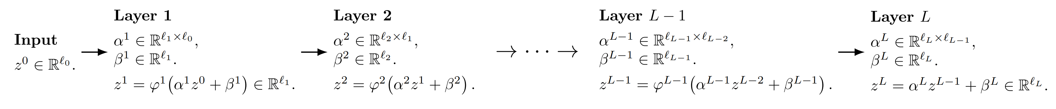
Figure 1: The framework for neural neural network.</div><p>The parameters we need to optimize can be listed as<br>$$<br>\Psi=\left((\alpha^1,\beta^1),(\alpha^2,\beta^2),\cdots,(\alpha^L,\beta^L)\right)\in \Pi=\left((\mathbb{R}^{l_1\times l_0}\times \mathbb{R}^{l_1})\times (\mathbb{R}^{l_2\times l_1}\times \mathbb{R}^{l_2})\times \cdots \times (\mathbb{R}^{l_L\times l_{L-1}}\times \mathbb{R}^{l_L})\right).<br>$$<br>And the reconstruction map can be defined as<br>$$<br>\begin{aligned}<br>\operatorname{R\Psi}: \mathbb{R}^{l_0}&amp;\to \mathbb{R}^{l_L}\\\<br>z^0&amp;\mapsto z^L.<br>\end{aligned}<br>$$<br>And the learning task can be formulated as the following optimization problem (often <strong>non-convex</strong>)<br>$$<br>\inf_{\Psi\in\Pi} \int_{\mathbb{R}^{l_0}\times \mathbb{R}^{l_L}} \Phi\Big(y-(\operatorname{R\Psi})(z)\Big)\  \nu(dz,dy),<br>$$<br>where $\Phi: \mathbb{R}^{l_L}\to \mathbb{R}$ is a convex function.</p><h3 id="Two-Layer-Neural-Networks"><a href="#Two-Layer-Neural-Networks" class="headerlink" title="Two Layer Neural Networks"></a>Two Layer Neural Networks</h3><p>Now we focus on the two layer neural networks. Let $l_0=d-1,L=2, l_1=n, l_2=1$ and $\beta^1=\beta^2=0$. We can partition the matrix $\alpha^1\in \mathbb{R}^{n\times (d-1)}$ into blocks<br>$$<br>\alpha^1=\begin{pmatrix}<br>(\alpha_1^1)^T\\\<br>(\alpha_2^1)^T\\\<br>\vdots\\\<br>(\alpha_n^1)^T<br>\end{pmatrix},\quad \alpha_i^1\in \mathbb{R}^{d-1},\ i=1,2,\cdots,n<br>$$<br>and let<br>$$<br>\alpha^2=\Big(\frac{c_1}{n},\frac{c_2}{n},\cdots,\frac{c_n}{n}\Big),\quad c_i\in \mathbb{R},\ i=1,2,\cdots,n.<br>$$<br>Then for input $z^0\in \mathbb{R}^{d-1}$, we have<br>$$<br>z^1=\varphi^n(\alpha^1 z^0)=\begin{pmatrix}<br>\varphi(\alpha_1^1\cdot z^0)\\\<br>\varphi(\alpha_2^1\cdot z^0)\\\<br>\vdots\\\<br>\varphi(\alpha_n^1\cdot z^0)<br>\end{pmatrix}<br>$$<br>and<br>$$<br>z^2=\alpha^2z^1=\frac{1}{n}\sum_{i=1}^n c_i\varphi(\alpha_i^1\cdot z^0),<br>$$<br>where “$\cdot$” denotes the inner product. Hence the reconstruction map for two layer neural networks problem is<br>$$<br>\begin{aligned}<br>\operatorname{R\Psi}: \mathbb{R}^{d-1}&amp;\to \mathbb{R}\\\<br>z&amp;\mapsto \frac{1}{n}\sum_{i=1}^n c_i\varphi(\alpha_i^1\cdot z).<br>\end{aligned}<br>$$<br>Then the learning task can be formulated as the following optimization problem (often <strong>non-convex</strong>)<br>$$<br>\inf_{\alpha_i,\ c_i,\  i=1,2,\cdots,n} \int_{\mathbb{R}^{d}} \Phi\Big(y-\frac{1}{n}\sum_{i=1}^n c_i\varphi(\alpha_i\cdot z)\Big)\  \nu(dz,dy),<br>$$<br>where $\Phi: \mathbb{R}\to \mathbb{R}$ is a convex function. To simplify the notations, we denote $x=(\alpha,c)\in \mathbb{R}^{d}$ and<br>$$<br>\widehat\varphi (x,z):= c\varphi(\alpha\cdot z).<br>$$<br>Then the optimization problem can be written as<a id="problem1"></a><br>$$<br>\inf_{x^i=(\alpha_i,c_i),\  i=1,2,\cdots,n} F^n(x^1,\cdots,x^n):= \int_{\mathbb{R}^{d}} \Phi\Big(y-\frac{1}{n}\sum_{i=1}^n \widehat\varphi(x^i,z)\Big)\  \nu(dz,dy).\tag{P1}<br>$$<br><strong>One of the most important observation is that if we lift the finite-dimensional optimization problem <a href="#problem1">(P1)</a> to the infinite-dimensional optimization problem over the space of probability measures <a href="#problem2">(P2)</a><a id="problem2"></a>, it will become convex.</strong><br>$$<br>\inf_{m\in \mathcal{P}(\mathbb{R}^d)} F(m):=\int_{\mathbb{R}^{d}} \Phi\Big(y-\mathbb{E}_{X\sim m}[\widehat\varphi(X,z)]\Big)\  \nu(dz,dy).\tag{P2}<br>$$</p><p><strong>Proposition 1.</strong> The functional $F: \mathcal{P}(\mathbb{R}^d)\to\mathbb{R}$ is convex.</p><p><strong><em>Proof</em></strong> : For all $m,m^\prime\in \mathcal{P}(\mathbb{R}^d)$ and all $t\in [0,1]$, </p><p>$$<br>\begin{aligned}<br>F((1-t)m+tm^\prime) &amp;=\int_{\mathbb{R}^{d}} \Phi\Big(y-\mathbb E_{X\sim (1-t)m+tm^\prime}[\widehat\varphi(X,z)]\Big)\  \nu(dz,dy)\\\<br>&amp;=\int_{\mathbb{R}^{d}} \Phi\Big((1-t)(y-\mathbb E_{X\sim m}[\widehat\varphi(X,z)])+t(y-\mathbb E_{X\sim m^\prime}[\widehat\varphi(X,z)])\Big)\  \nu(dz,dy)\\\<br>&amp;\le (1-t)\int_{\mathbb{R}^{d}} \Phi\Big(y-\mathbb E_{X\sim m}[\widehat\varphi(X,z)]\Big)\  \nu(dz,dy)+t \int_{\mathbb{R}^{d}} \Phi\Big(y-\mathbb E_{X\sim m^\prime}[\widehat\varphi(X,z)]\Big)\  \nu(dz,dy)\\\<br>&amp;=(1-t)F(m)+tF(m^\prime).<br>\end{aligned}<br>$$</p><p>Hence $F$ is convex. $\square$</p><p>Now maybe you want to ask what is the relationship between <a href="#problem1">(P1)</a> and <a href="#problem2">(P2)</a> ? It is obvious that<br>$$<br>F^n(x^1,\cdots,x^n)=F(\frac{1}{n}\sum_{i=1}^n \delta_{x^i}).<br>$$<br>Hence we have<br>$$<br>\inf_{x^i,\  i=1,2,\cdots,n} F^n(x^1,\cdots,x^n)\ge \inf_{m\in \mathcal{P}(\mathbb{R}^d)} F(m).<br>$$<br>Moreover,we have the following theorem, which shows that the infimum of  <a href="#problem1">(P1)</a> and <a href="#problem2">(P2)</a> is very close as long as $n$ is sufficiently large.</p><p><strong>Theorem 1.</strong> <a id="theorem1"></a> We assume that the 2nd order linear functional derivative of $F$ exists, is jointly continuous in both variables and that there is $L&gt;0$ such that for any random variables $\eta_1,\eta_2$ such that $\mathbb{E}[|\eta_i|^2]&lt;\infty$, $i=1,2$, it holds that</p><p>$$<br>\mathbb{E} \left[\sup_{\nu\in\mathcal P_2(\mathbb{R}^d)}\left\vert\frac{\delta F}{\delta m}(\nu,\eta_1)\right\vert\right]<br>+<br>\mathbb{E}\left[\sup_{\nu\in\mathcal P_2(\mathbb{R}^d)}\left\vert\frac{\delta^2 F}{\delta m^2}(\nu,\eta_1,\eta_2)\right\vert\right]<br>\leq L<br>$$</p><p>If there is an $m^\star\in\mathcal P_2(\mathbb{R}^d)$ such that $F(m^\star)=\inf_{m\in\mathcal P_2(\mathbb{R}^d)}F(m)$ then we have that</p><p>$$<br>\left|<br>\inf_{x^i,\  i=1,2,\cdots,n}<br>F\left(\frac{1}{n}\sum_{i=1}^n\delta_{x^i}\right)<br>-<br>F(m^\star)<br>\right|<br>\leq<br>\frac{2L}{n}.<br>$$</p><hr><p>So the question becomes how to solve  <a href="#problem2">(P2)</a>? From now on, we assume the functional $F$ has the following properties.</p><p><strong>Assumption 1.</strong> <a id="assumption1"></a> Assume that $F \in \mathcal C^1$ is convex and bounded from below, where we say a function $F : \mathcal{P}(\mathbb{R}^d) \to \mathbb{R}$ is in $\mathcal C^1$ if there exists a bounded continuous function<br>$$<br>\frac{\delta F}{\delta m} : \mathcal{P}(\mathbb{R}^d) \times \mathbb{R}^d \to \mathbb{R}<br>$$<br>such that<a id="equation1"></a><br>$$<br>F(m’) - F(m) = \int_0^1 \int_{\mathbb{R}^d} \frac{\delta F}{\delta m}\bigl((1-\lambda)m + \lambda m’, x\bigr)\ (m’ - m)(dx)\ d\lambda.<br>\tag{1}<br>$$</p><p>We will refer to $\frac{\delta F}{\delta m}$ as the linear functional derivative. There is at most one $\frac{\delta F}{\delta m}$, up to a constant shift, satisfying <a href="#equation1">(1)</a>. To avoid the ambiguity, we impose<br>$$<br>\int_{\mathbb{R}^d} \frac{\delta F}{\delta m}(m,x)\ m(dx)=0.<br>$$</p><p>If $(m,x)\mapsto \frac{\delta F}{\delta m}(m,x)$ is continuously differentiable in $x$, we define its intrinsic derivative $D_m F : \mathcal{P}(\mathbb{R}^d)\times \mathbb{R}^d \to \mathbb{R}^d$ by<br>$$<br>D_m F(m,x)=\nabla\left(\frac{\delta F}{\delta m}(m,x)\right).<br>$$</p><p>However, even under the <a href="#assumption1">Assumption 1</a>, the existence and uniqueness of the minimizer of the optimization problem <a href="#problem2">(P2)</a> is not clear. So instead, we can consider the regularized problem <a href="#problem3">(P3)</a>.<a id="problem3"></a></p><p>$$<br>\inf_{m\in \mathcal{P}(\mathbb{R}^d)} V^\sigma(m):=F(m)+\frac{\sigma^2}{2}H(m),\tag{P3}<br>$$<br>where<br>$$<br>g(x)=e^{-U(x)} \text{ with } U \text{ s.t. } \int_{\mathbb{R}^d} e^{-U(x)}dx=1,<br>$$<br>is the density of the Gibbs measure and the function $U$ satisfies the following conditions.</p><p><strong>Assumption 2.</strong> <a id="assumption2"></a>The function $U:\mathbb{R}^d \to \mathbb{R}$ belongs to $C^\infty$. Further,</p><p>(i) there exist constants $C_U&gt;0$ and $C’_U\in\mathbb{R}$ such that<br>$$<br>\nabla U(x)\cdot x \ge C_U |x|^2 + C’_U \quad \text{for all } x\in\mathbb{R}^d.<br>$$<br>(ii) $\nabla U$ is Lipschitz continuous.</p><p>Immediately, we obtain that there exist $0\le C’ \le C$ such that for all $x\in\mathbb{R}^d$<br>$$<br>C’|x|^2 - C \le U(x) \le C(1+|x|^2), \qquad |\Delta U(x)| \le C.<br>$$</p><p>For regularized optimization problem <a href="#problem3">(P3)</a>, we have a necessary and sufficient first-order optimality condition.</p><p><strong>Theorem 2.</strong> <a id="theorem2"></a> Under <a href="#assumption1">Assumptions 1</a> and <a href="#assumption2">Assumption 2</a>, the function $V^\sigma$ has a unique minimizer absolutely continuous with respect to Lebesgue measure $\ell$, and belonging to $\mathcal{P}_2(\mathbb{R}^d)$. Moreover,<br>$$<br>m^* \in \mathcal{P}_2(\mathbb{R}^d) = \underset{m \in \mathcal{P}(\mathbb{R}^d)}{\arg\min}\  V^\sigma(m)<br>$$<br>if and only if $m^*$ is equivalent to Lebesgue measure and<a id="equation2"></a></p><p>$$<br>\frac{\delta F}{\delta m}(m^\star, \cdot) + \frac{\sigma^2}{2} \log(m^\star) + \frac{\sigma^2}{2} U<br>\text{ is a constant, } \ell\text{-a.s.},<br>\tag{2}<br>$$</p><p>where we abuse the notation, still denoting by $m^*$ the density with respect to Lebesgue measure.</p><p>What’s more, as shown in <a href="https://handsteinwang.github.io/2026/02/18/An-Important-Example-of-Gamma-Convergence/">my previous blog: An Example of Gamma Convergence</a>, we know that<br>$$<br>V^\sigma = F + \frac{\sigma^2}{2} H \xrightarrow{\Gamma} F \quad\text{as } \sigma \downarrow 0.<br>$$<br>Therefore, every cluster point of<br>$$<br>\left(\arg\min_m V^\sigma(m)\right)_\sigma<br>$$<br>is a minimizer of $F$.</p><hr><p>By <a href="#theorem2">Theorem 2</a>, we know that if $m^\star$ is the unique minimizer of <a href="#problem3">(P3)</a>, then<a id="equation3"></a><br>$$<br>D_m F(m^\star, x) + \frac{\sigma^2}{2} \frac{\nabla m^\star(x)}{m^\star(x)} + \frac{\sigma^2}{2} \nabla U(x)<br>=0\quad \ell\text{-a.s.},<br>\tag{3}<br>$$<br>which means $m^\star$ is the invariant measure of the following Fokker-Planck equation<a id="equation4"></a><br>$$<br>\partial_t m_t=\nabla\cdot \left[\left(D_m F(m_t, x)+\frac{\sigma^2}{2} \nabla U(x)\right)m_t\right]+\frac{\sigma^2}{2}  \Delta m_t.\tag{4}<br>$$</p><p>Therefore, $m^\star$ is also the invariant measure of the following mean-field Langevin dynamic<a id="equation5"></a><br>$$<br>dX_t = -\left(D_m F(m_t,X_t) + \frac{\sigma^2}{2}\nabla U(X_t)\right)dt + \sigma dW_t,<br>\qquad \text{where } m_t := \mathrm{Law}(X_t).<br>\tag{5}<br>$$</p><hr><p>However, the dynamic <a href="#equation5">(5)</a> is hard to discretization. Consider independent random variables $X_0^i$, $X_0^i\sim m_0$ and independent Brownian motions $(W^i),\ i=,1,2\cdots,n$. By approximating the law of the process <a href="#equation5">(5)</a> its empirical law we arrive at the following interacting particle system<a id="equation6"></a></p><p>$$<br>\begin{cases}<br>dX_t^i=-\left(D_mF(m_t^n,X_t^i)+\frac{\sigma^2}{2}\nabla U(X_t^i)\right)dt+\sigma dW_t^i,\quad i=1,\ldots,n,\\\<br>m_t^n=\dfrac{1}{n} \sum\limits_{i=1}^n\delta_{X_t^i}.<br>\end{cases}<br>\tag{6}<br>$$<br>By the theory of mean-field limit, we know as $n\to\infty$, the dynamic <a href="#equation6">(6)</a> will tend to dynamic <a href="#equation5">(5)</a>. By the following lemma, the term $D_mF(m_t^n,X_t^i)$ is easy to compute.</p><p><strong>Lemma 1.</strong> <a id="lemma1"></a> We have<br>$$<br>\partial_{x^i} F^n(x^1,\cdots,x^n) = \frac{1}{n}D_mF(\sum_{i=1}^n \delta_{x^i},x^i).<br>$$</p><p>Hence by <a href="#lemma1">Lemma 1</a>, the dynamic <a href="#equation6">(6)</a> can be written as<br>$$<br>dX_t^i = -\left( n \partial_{x_i} F^n(X_t^1,\cdots,X_t^n) + \frac{\sigma^2}{2} \nabla U(X_t^i) \right) dt + \sigma dW_t^i .\quad i=1,2,\cdots,n.<br>$$<br>By the definition of $F^n$ in <a href="#problem1">(P1)</a>, we have<br>$$<br>\partial_{x^i} F^n(x^1,\cdots,x^n)<br>=<br>-\frac{1}{n}<br>\int_{\mathbb{R}^d}<br>\dot{\Phi}!\left(<br>y-\frac{1}{n}\sum_{j=1}^n \hat{\varphi}(x^j,z)<br>\right)<br>\nabla \hat{\varphi}(x^i,z)\ \nu(dz,dy).<br>$$</p><p>We thus see that the dynamic <a href="#equation6">(6)</a> corresponds to</p><p>$$<br>dX_t^i<br>=<br>\left(<br>\int_{\mathbb{R}^d}<br>\Phi^\prime\left(<br>y-\frac{1}{n}\sum_{j=1}^n \hat{\varphi}(X_t^j,z)<br>\right)<br>\nabla \hat{\varphi}(X_t^i,z)\ \nu(dz,dy)<br>-<br>\frac{\sigma^2}{2}\nabla U(X_t^i)<br>\right)dt<br>+\sigma dW_t^i ,\quad i=1,2,\cdots,n.<br>$$</p><p>For a fixed time step $\tau &gt; 0$ fixing a grid of time points $t_k = k\tau$, $k = 0,1,\ldots$ we can then write the explicit Euler scheme</p><p>$$<br>X_{t_{k+1}}^{\tau,i} - X_{t_k}^{\tau,i}<br>=<br>\left(<br>\int_{\mathbb{R}^d}<br>\Phi^\prime \left(<br>y - \frac{1}{n}\sum_{j=1}^n \hat{\varphi}(X_{t_k}^{\tau,j},z)<br>\right)<br>\nabla \hat{\varphi}(X_{t_k}^{\tau,i},z)\ \nu(dz,dy)<br>-<br>\frac{\sigma^2}{2}\nabla U(X_{t_k}^{\tau,i})<br>\right)\tau<br>+<br>\sigma\bigl(W_{t_{k+1}}^i - W_{t_k}^i\bigr).<br>$$</p><p>To relate this to the gradient descent algorithm we consider the case where we are given data points $(y_m,z_m),\ m=1,2,\cdots,N$ which are i.i.d. samples from $\nu$. If the loss function $\Phi(x)=x^2$ is simply the square loss then the evolution of parameter $x_k^i$ will simply read as</p><p>$$<br>x_{k+1}^i<br>=<br>x_k^i<br>+<br>2\tau<br>\left(<br>\left(<br>y_{I_k} - \frac{1}{n}\sum_{j=1}^n \hat{\varphi}(x_k^j,z_{I_k})<br>\right)<br>\nabla \hat{\varphi}(x_k^i,z_{I_k})<br>-<br>\frac{\sigma^2}{2}\nabla U(x_k^i)<br>\right)<br>+<br>\sigma\sqrt{\tau}\ \xi_k^i,<br>$$</p><p>with$I_k\sim \mathrm{Unif}\{1,2,\cdots,N\}$ and  $\xi_k^i$ independent samples from $N(0,I_d)$, which can be viewed as a version of <strong>regularized noisy SGD algorithm</strong>.</p><h2 id="Summary"><a href="#Summary" class="headerlink" title="Summary"></a>Summary</h2><p>The main analytical framework of this theory can be illustrated by the following diagram.<a id="fig2"></a></p><div align="center">  <img src="/images/meanfield_intro.png" style="zoom:100%; display:block; margin:0 auto;" />  
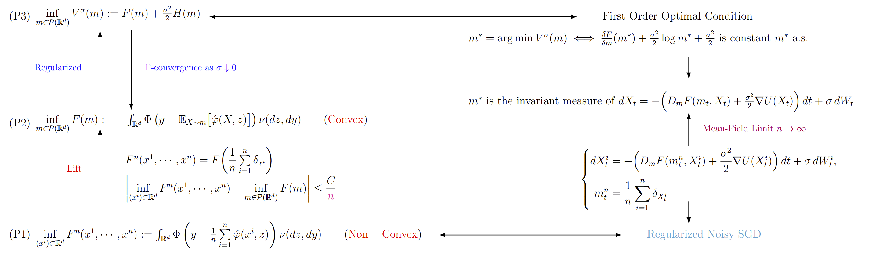
Figure 2: Summary of the main analytical framework.</div><h2 id="Reference"><a href="#Reference" class="headerlink" title="Reference"></a>Reference</h2><p>Hu, Kaitong, et al. “Mean-field Langevin dynamics and energy landscape of neural networks.” <em>Annales de l’Institut Henri Poincare (B) Probabilites et statistiques</em>. Vol. 57. No. 4. Institut Henri Poincaré, 2021. <a id="refhu"></a></p><blockquote><p>The cover image of this article was taken at Jungfrau in Switzerland.</p></blockquote>]]>
    </content>
    <id>https://handsteinwang.github.io/2026/03/25/An-Introduction-to-Mean-Field-Langevin-Dynamics/</id>
    <link href="https://handsteinwang.github.io/2026/03/25/An-Introduction-to-Mean-Field-Langevin-Dynamics/"/>
    <published>2026-03-24T16:00:00.000Z</published>
    <summary>
      <![CDATA[<p>Optimization over the space of probability measures is not only widely applicable, but also offers a useful perspective for analyzing certain complicated finite-dimensional nonconvex optimization problems. In particular, lifting such problems to optimization problems over probability measures can lead to better structural properties, such as convexity. Mean-field Langevin dynamics provides a representative example of this idea. Its central motivation is that some highly nonconvex optimization problems arising in neural network training become better behaved when reformulated as the optimization of a functional on the space of probability measures. This viewpoint also makes it possible to build a theoretical foundation for understanding the convergence of SGD. In what follows, we briefly introduce this perspective, mainly based on the paper by <a href="#refhu">[Hu, Kaitong, et al]</a>. The main analytical framework of this theory can be illustrated by <a href="#fig2">Figure 2</a>.</p>]]>
    </summary>
    <title>An Introduction to Mean-Field Langevin Dynamics</title>
    <updated>2026-03-26T16:00:00.000Z</updated>
  </entry>
  <entry>
    <author>
      <name>Handstein Wang</name>
    </author>
    <category term="Probability Theory" scheme="https://handsteinwang.github.io/categories/Probability-Theory/"/>
    <category term="Probability Theory" scheme="https://handsteinwang.github.io/tags/Probability-Theory/"/>
    <category term="Measure Theory" scheme="https://handsteinwang.github.io/tags/Measure-Theory/"/>
    <content>
      <![CDATA[<p>In this article, we will introduce some important properties of the relative entropy, including lower semi-continuity, convexity, compactness of sublevel sets based on the Donsker-Varadhan variational formula.</p><span id="more"></span>    <p>Let $X$ be a Polish space, and $\mathcal{B}$ be the corresponding Borel $\sigma-$algebra. We denote by $\mathcal{P}(X)$ the set of probability measures on $(X,\mathcal{B})$.</p><p><strong>Definition 1.</strong> For $\nu\in \mathcal{P}(X)$, the relative entropy functional (also called KL divergence) is a mapping $H(\cdot \Vert\nu ): \mathcal{P}(X)\to \overline{\mathbb{R}}$, defined by</p><p>$$<br>H(\mu\Vert\nu):=\begin{cases}<br>\int_X \log \left(\frac{d\mu}{d\nu}\right)d\mu,&amp; \text{if } \mu\ll \nu\\\<br>+\infty,&amp; \text{otherwise}<br>\end{cases}.<br>$$</p><p><strong>Remark 1.</strong> Since $s(\log s)^{-}$ is bounded for $s\in [0,+\infty)$, whenever $\mu\in \mathcal{P}(X)$ is absolutely continuous with respect to $\nu$,</p><p>$$<br>\int_X \log \left(\frac{d\mu}{d\nu}\right)^{-}d\mu=\int_X \frac{d\mu}{d\nu}\log \left(\frac{d\mu}{d\nu}\right)^{-}d\nu&lt;+\infty.<br>$$</p><p>It follows that the relative entropy is well-defined.</p><p><strong>Lemma 1.</strong> For $\nu\in \mathcal{P}(X)$, the relative entropy $H(\cdot\Vert\nu)$ functional is positive definite, namely, $H(\mu\Vert\nu)\ge 0$ and $H(\mu\Vert\nu)=0$ if and only if $\mu=\nu$.</p><p><strong>Proof.</strong>  It suffices to consider the case where $H(\mu\Vert\nu)&lt;+\infty$. Since $s\log s\ge s-1$ with equality if and only if $s=1$,<br>$$<br>H(\mu\Vert\nu)=\int_X \frac{d\mu}{d\nu}\log \left(\frac{d\mu}{d\nu}\right) d\nu\ge \int_X  \left(\frac{d\mu}{d\nu}-1\right) d\nu=\int_X d\mu-\int_Xd\nu=\mu(X)-\nu(X)=0.<br>$$<br>And the equality holds if and only if<br>$$<br>\frac{d\mu}{d\nu}=1\quad \nu-a.e.\ ,<br>$$<br>if and only if $\mu=\nu$. This complete the proof. $\square$</p><p><strong>Proposition 1.</strong> Let $f:X\to\mathbb{R}$ be a bounded measurable function and $\nu\in \mathcal{P}(X)$. The following conclusions holds.</p><p>(a) We have the variational formula<br>$$<br>-\log \int_X e^{-f} d\nu=\inf_{\mu\in \mathcal{P}(X)} \left\{ H(\mu\Vert \nu)+\int_X f\  d\mu \right\}.\tag{1}<br>$$<br>(b) Let $\mu_0$ denotes the probability measure on $X$ which is absolutely continuous with respect to $\nu$ and satisfies<br>$$<br>\frac{d\mu_0}{d\nu}(x) = \frac{e^{-f(x)}}{\int_X e^{-f}d\nu}.<br>$$<br>Then the infimum in the variational formula (1) is uniquely attained at $\mu_0$.</p><p><strong>Proof.</strong> For part (a), it suffices to prove that<br>$$<br>-\log \int_X e^{-f} d\nu=\inf \left\{ H(\mu\Vert \nu)+\int_X f\  d\mu: \mu \in \mathcal{P}(X),\ H(\mu\Vert\nu)&lt;+\infty\right\}.<br>$$<br>If $H(\mu\Vert\nu)&lt;+\infty$, then $\mu\ll\nu$ and since by definition $\nu\ll \mu_0$, we have also $\mu\ll\mu_0$. Thus</p><p>$$<br>\begin{aligned}<br>H(\mu\Vert \nu)+\int_X f\  d\mu&amp;= \int_X \log \left(\frac{d\mu}{d\nu}\right)d\mu +\int_X f\  d\mu\\\<br>&amp;=\int_X \log \left(\frac{d\mu}{d\mu_0}\right)d\mu+\int_X \log \left(\frac{d\mu_0}{d\nu}\right)d\mu +\int_X f\  d\mu\\\<br>&amp;=H(\mu\Vert\mu_0)-\log \int_X e^{-f} d\nu.<br>\end{aligned}<br>$$<br>Hence by proposition 1, we complete the proof. $\square$</p><p>Now, we denote by $C_b(X)$ the space of bounded continuous functions mapping $X$ into $\mathbb{R}$ and by $B_b(X)$ the space of bounded Borel measurable functions mapping $X$ into $\mathbb{R}$. </p><p><strong>Theorem 1 (Donsker-Varadhan variational formula).</strong> For each $\mu$ and $\nu$ in $\mathcal{P}(X)$,<br>$$<br>H(\mu\Vert\nu)=\sup_{g\in C_b(X)}\left\{\int_X g\ d\mu-\log\int_X e^{g}\ d\nu\right\}=\sup_{h\in B_b(X)}\left\{\int_X h\ d\mu-\log\int_X e^{h}\ d\nu\right\}.<br>$$</p><p><strong>Proof.</strong> We first show that<br>$$<br>\sup_{g\in C_b(X)}\left\{\int_X g\ d\mu-\log\int_X e^{g}\ d\nu\right\}=\sup_{h\in B_b(X)}\left\{\int_X h\ d\mu-\log\int_X e^{h}\ d\nu\right\}.<br>$$<br>On the one hand, given $\varepsilon&gt;0$, since $X$ is a Polish space, $\mu$ and $\nu$ are Borel probability measure, by Ulam’s Theorem, $\mu$ and $\nu$ are tight. Hence, there is a compact subset $K$ of $X$ such that<br>$$<br>\mu(K^c)\le \varepsilon\quad \text{and}\quad \nu(K^c)\le \varepsilon.<br>$$<br>By Lusin’s Theorem and the Tietze-Urysohn Extension Theorem, for any $h\in B_b(X)$, there exists a closed subset $F$ of $K$, which is also compact, such that<br>$$<br>\mu(K\setminus F)\le \varepsilon \quad \text{and}\quad \nu(K\setminus F)\le \varepsilon.<br>$$<br>And $g\in C_b(X)$ such that</p><p>$$<br>g|_F=h|_F<br>$$</p><p>and<br>$$<br>\lVert g\rVert_{\infty}\le \lVert h\rVert_{\infty}.<br>$$<br>It follows that<br>$$<br>\mu(F^c)\le \mu(K^c)+ \mu(K\setminus F)\le 2\varepsilon \quad \text{and}\quad \nu(F^c)\le \nu(K^c)+ \nu(K\setminus F)\le 2\varepsilon<br>$$<br>and that<br>$$<br>\begin{aligned}<br>\int_X h\ d\mu-\log\int_X e^{h}\ d\nu &amp;=\int_{F} h\ d\mu-\log\int_{F} e^{h}\ d\nu+\int_{F^c} h\ d\mu-\log\int_{F^c} e^{h}\ d\nu\\\<br>&amp;\le \int_{F} g\ d\mu-\log\int_{F} e^{g}\ d\nu+4\lVert h\rVert_{\infty}\varepsilon\\\<br>&amp;=\int_{X} g\ d\mu-\log\int_{X} e^{g}\ d\nu-\int_{F^c} g\ d\mu+\log\int_{F^c} e^{g}\ d\nu+4\lVert h\rVert_{\infty}\varepsilon\\\<br>&amp;\le \int_{X} g\ d\mu-\log\int_{X} e^{g}\ d\nu+ 8\lVert h\rVert_{\infty}\varepsilon.<br>\end{aligned}<br>$$</p><p>Taking the supremum over $g\in C_b(X)$ and letting $\varepsilon\to 0$ yields<br>$$<br>\int_X h\ d\mu-\log\int_X e^{h}\ d\nu \le \sup_{g\in C_b(X)}\left\{\int_X g\ d\mu-\log\int_X e^{g}\ d\nu\right\},<br>$$<br>and since $h\in B_b(X)$ is arbitrary, we conclude that<br>$$<br>\sup_{h\in B_b(X)}\left\{\int_X h\ d\mu-\log\int_X e^{h}\ d\nu\right\}\le \sup_{g\in C_b(X)}\left\{\int_X g\ d\mu-\log\int_X e^{g}\ d\nu\right\}.<br>$$<br>On the other hand, since $C_b(X)\subset B_b(X)$, we have<br>$$<br>\sup_{h\in B_b(X)}\left\{\int_X h\ d\mu-\log\int_X e^{h}\ d\nu\right\}\ge \sup_{g\in C_b(X)}\left\{\int_X g\ d\mu-\log\int_X e^{g}\ d\nu\right\}.<br>$$<br>Hence<br>$$<br>\sup_{g\in C_b(X)}\left\{\int_X g\ d\mu-\log\int_X e^{g}\ d\nu\right\}=\sup_{h\in B_b(X)}\left\{\int_X h\ d\mu-\log\int_X e^{h}\ d\nu\right\}.<br>$$<br>Next, we denote<br>$$<br>R(\mu,\nu):=\sup_{g\in C_b(X)}\left\{\int_X g\ d\mu-\log\int_X e^{g}\ d\nu\right\}=\sup_{h\in B_b(X)}\left\{\int_X h\ d\mu-\log\int_X e^{h}\ d\nu\right\}<br>$$<br>and we need to show<br>$$<br>R(\mu,\nu)=H(\mu\Vert \nu).<br>$$<br>Since the function $g_0\equiv 0$ on $X$ is also bounded continuous, we have<br>$$<br>R(\mu,\nu)\ge\int_X g_0\ d\mu-\log\int_X e^{g_0}\ d\nu=0.<br>$$<br>By Proposition 1, for any $f\in B_b(X)$,<br>$$<br>H(\mu\Vert\nu)\ge -\int_X f\ d\mu-\log \int_X e^{-f}\ d\nu.<br>$$<br>Replacing $f$ by $h:=-f$, and taking the supremum over $h\in B_b(X)$, we obtain<br>$$<br>H(\mu\Vert\nu)\ge\sup_{h\in B_b(X)}\left\{\int_X h\ d\mu-\log\int_X e^{h}\ d\nu\right\}=R(\mu,\nu).<br>$$<br>Now, we only need to show that<br>$$<br>R(\mu,\nu)\ge H(\mu\Vert\nu).<br>$$<br>We may assume that $R(\mu,\nu)&lt;+\infty$ for otherwise there is nothing to prove. </p><p>We claim that under this condition, $\mu\ll\nu$. Indeed, let $A\in \mathcal{B}$ such that $\nu(A)=0$ and take $h=r1_A$ with $r&gt;0$, we have<br>$$<br>r\mu(A)=\int_X h\ d\mu-\log\int_X e^{h}\ d\nu\le R(\mu,\nu)&lt;\infty.<br>$$<br>Taking $r\to\infty$ gives $\mu(A)=0$ as claimed.</p><p>Since $\mu\ll\nu$, the Radon-Nikodym derivative<br>$$<br>f:=\frac{d\mu}{d\nu}<br>$$<br>exists. </p><p>Case 1: $f(x)&gt;0$ for all $x\in X$ and bounded. Then $h=\log f$ is bounded and measurable. Hence by<br>$$<br>\log\int_X e^{h}\ d\nu=\log\int_X f\ d\nu=\log\int_X d\mu=0,<br>$$</p><p>we have</p><p>$$<br>H(\mu\Vert \nu)=\int_X \log f\  d\mu= \int_X h\  d\mu- \log\int_X e^{h}\ d\nu \le R(\mu,\nu).<br>$$<br>Case 2: $f(x)&gt;0$ for all $x\in X$ but $f$ is not bounded. Then for $n\in \mathbb{N}$, we set $f_n=f\wedge n$ and $h=\log f_n$, we obtain by Monotone Convergence Theorem<br>$$<br>H(\mu\Vert \nu)=\int_X \log f\  d\mu=\lim_{n\to\infty}\int_X \log f_n\  d\mu\le R(\mu,\nu)+\lim_{n\to\infty} \log\int_X f_n\  d\nu=R(\mu,\nu).<br>$$<br>Case 3: neither $f(x)&gt;0$ for all $x\in X$ nor bounded. For $t\in [0,1]$, define<br>$$<br>\mu_t:=t\nu+(1-t)\mu\quad\text{and}\quad f_t:= \frac{d\mu_t}{d\nu}=t\cdot 1+(1-t)f.<br>$$<br>For each $t\in (0,1]$, $f_t&gt;0$ for all $x\in X$ and so by Case 2, we have<br>$$<br>H(\mu_t\Vert\nu)\le R(\mu_t,\nu).<br>$$<br>We now prove that<br>$$<br>\lim_{t\to 0} H(\mu_t\Vert\nu)=H(\mu\Vert\nu)\quad \text{and}\quad \lim_{t\to 0}R(\mu_t,\nu)=R(\mu,\nu),<br>$$<br>which will complete the proof.</p><p>Since $s\log s$ is convex on $[0,+\infty)$,<br>$$<br>H(\mu_t\Vert \nu)=\int_X f_t\log f_t\ d\nu\le (1-t) \int_X f\log f\ d\nu=(1-t)H(\mu\Vert \nu).<br>$$<br>Therefore,<br>$$<br>\limsup_{t\to 0} H(\mu_t\Vert \nu)\le H(\mu\Vert \nu).<br>$$</p><p>Moreover, since $f_t\ge t$ we have $\log f_t\ge \log t$ and $\log s$ is concave, we have<br>$$<br>\log f_t\ge (1-t)\log f,<br>$$</p><p>which follows that<br>$$<br>H(\mu_t\Vert \nu)=\int_X f_t\log f_t\ d\nu=t\int_X \log f_t \ d\nu+(1-t) \int_X f\log f_t\ d\nu\ge t\log t +(1-t)^2 H(\mu\Vert\nu).<br>$$<br>Therefore,<br>$$<br>\liminf_{t\to 0} H(\mu_t\Vert \nu)\ge H(\mu\Vert \nu).<br>$$</p><p>Thus we have<br>$$<br>\lim_{t\to 0} H(\mu_t\Vert \nu)=H(\mu\Vert \nu).<br>$$<br>For $R(\mu,\nu)$, by Jensen’s inequality, for $g\in C_b(X)$,<br>$$<br>-\log\int_X e^g\  d\nu\le \int_X (-\log e^g)\  d\nu=-\int_X g\ d\nu,<br>$$<br>which follows that<br>$$<br>0\le R(\nu,\nu)=\sup_{g\in C_b(X)}\left\{\int_X g\ d\nu-\log\int_X e^{g}\ d\nu\right\}\le 0.<br>$$<br>Therefore $R(\nu,\nu)=0$. It is easy to check that the mapping $t\in [0,1]\mapsto R(\mu_t,\nu)$ is convex and lower semi-continuous. Furthermore,<br>$$<br>0\le R(\mu_t,\nu)\le tR(\nu,\nu)+(1-t) R(\mu,\nu)=(1-t) R(\mu,\nu)\le  R(\mu,\nu)&lt;+\infty<br>$$<br> and so it is also bounded. By convex analysis, we know that $t\in [0,1]\mapsto R(\mu_t,\nu)$ is continuous and therefore<br>$$<br>\lim_{t\to 0}R(\mu_t,\nu)=R(\mu,\nu).<br>$$<br>This complete the proof. $\square$</p><p><strong>Theorem 2.</strong> The relative entropy $H(\mu\Vert \nu)$ is a convex, lower semi-continuous function of $(\mu,\nu)\in \mathcal{P}(X)\times \mathcal{P}(X)$. In particular, $H(\mu\Vert \nu)$ is a convex, lower semi-continuous function of each $\mu$ and $\nu$ separately. In addition, for fixed $\nu\in \mathcal{P}(X)$, the relative entropy $H(\cdot\Vert\nu)$ is strictly convex on the set<br>$$<br>\{\mu\in \mathcal{P}(X): H(\mu\Vert\nu)&lt;+\infty\}.<br>$$</p><p><strong>Proof.</strong> By Donsker-Varadhan variational formula, we have<br>$$<br>H(\mu\Vert\nu)=\sup_{g\in C_b(X)}\left\{\int_X g\ d\mu-\log\int_X e^{g}\ d\nu\right\}.<br>$$<br>Since for each fixed $g\in C_b(X)$, the mapping<br>$$<br>(\mu,\nu)\in \mathcal{P}(X)\times \mathcal{P}(X)\mapsto \int_X g\ d\mu-\log\int_X e^{g}\ d\nu<br>$$<br>is convex and continuous. As the supremum over $g\in C_b(X)$, we have $H(\mu\Vert \nu)$ is a convex, lower semi-continuous function of $(\mu,\nu)\in \mathcal{P}(X)\times \mathcal{P}(X)$.</p><p>To prove the strict convexity on<br>$$<br>\{\mu\in \mathcal{P}(X): H(\mu\Vert\nu)&lt;+\infty\},<br>$$<br>where we have<br>$$<br>H(\mu\Vert\nu)=\int_X \frac{d\mu}{d\nu}\log \left(\frac{d\mu}{d\nu}\right) d\nu.<br>$$<br>Then the strict convexity follows from the strict convexity of $s\log s$ for $s\in [0,+\infty)$. This complete the proof. $\square$</p><p><strong>Remark.</strong> The relative entropy is often not continuous even with respect to the strong convergence of probability measures.</p><p><strong>Conterexample.</strong> Let<br>$$<br>\mu_n:=\frac{1}{a_n}\operatorname{Unif}[1,n]+\left(1-\frac{1}{a_n}\right)\operatorname{Unif}[-2,-1],<br>$$<br>where $a_n=\log\log n$ and<br>$$<br>\mu:=\operatorname{Unif}[-2,-1].<br>$$<br>Then it is easy to show that<br>$$<br>\operatorname{TV}(\mu_n,\mu)=\frac{1}{a_n}\to 0.<br>$$<br>However, let $\gamma$ be the Gaussian measure on $\mathbb{R}$, then it is easy to show that<br>$$<br>H(\mu_n\Vert \gamma)\to +\infty\neq H(\mu\Vert \gamma)\quad \text{as } n\to\infty.<br>$$</p><p><strong>Theorem 3.</strong> For each $\nu\in \mathcal{P}(X)$, the relative entropy has compact sublevel sets. That is, for each $M&lt;+\infty$ the sublevel set<br>$$<br>\{\mu\in \mathcal{P}(X): H(\mu\Vert\nu)\le M\}<br>$$<br>is a compact subset of $\mathcal{P}(X)$.</p><p><strong>Proof.</strong> Let $\{\mu_n,\ n\in \mathbb{N}\}$ be any sequence in the sublevel set<br>$$<br>\{\mu\in \mathcal{P}(X): H(\mu\Vert\nu)\le M\},<br>$$<br>which implies<br>$$<br>\sup_{n\in \mathbb{N}} H(\mu_n\Vert \nu)\le M&lt;+\infty.<br>$$<br>By Donsker-Varadhan variational formula, for any $h\in B_b(X)$, we have for each $n\in \mathbb{N}$<br>$$<br>\int_X h\ d\mu_n-\log\int_X e^h\ d\nu\le H(\mu_n\Vert \nu)\le M.<br>$$</p><p>Let $\delta&gt;0$ and $\varepsilon&gt;0$ be given. Since $\nu$ is a Borel probability measure on Polish space $X$, by Ulam’s Theorem, $\nu$ is tight, which means there exists a compact set $K$ such that<br>$$<br>\nu(K^c)\le \delta.<br>$$<br>Take<br>$$<br>h(x)=\begin{cases}<br>0,&amp; x\in K\\\<br>\log (1+\frac{1}{\delta}),&amp; x\in K^c<br>\end{cases},<br>$$<br>which is bounded and Borel measurable, we have for each $n\in \mathbb{N}$,<br>$$<br>\int_X h\ d\mu_n-\log\int_X e^h\ d\nu=\log (1+\frac{1}{\delta})\ \mu_n(K^c)-\log\nu(K)-\log  \left[(1+\frac{1}{\delta})\nu(K^c)\right] \le M.<br>$$<br>It follows that<br>$$<br>\mu_n(K^c)\le \frac{1}{\log (1+\frac{1}{\delta})} \left(M+\log \left[ \nu(K)+(1+\frac{1}{\delta}) \nu(K^c)\right]\right)\le \frac{M+\log 2}{\log (1+\frac{1}{\delta})}.<br>$$<br>Hence we can choose $\delta&gt;0$ such that<br>$$<br>\frac{M+\log 2}{\log (1+\frac{1}{\delta})}\le \varepsilon,<br>$$</p><p>which implies that $\{\mu_n,\ n\in \mathbb{N}\}$ is tight. By Prohorov’s Theorem, there exists $\mu\in \mathcal{P}(X)$ and a subsequence $\mu_{n_k}$ such that $\mu_{n_k}$ weak converge to $\mu$. The lower semi-continuity of $H(\cdot\Vert\nu)$ yields<br>$$<br>H(\mu\Vert\nu)\le\liminf_{k\to\infty} H(\mu_{n_k}\Vert\nu)\le M,<br>$$<br>which means $\mu$ also lies in the sublevel set. This complete the proof. $\square$ </p><blockquote><p>The cover image of this article was taken while taking a helicopter sightseeing flight over Aoraki / Mount Cook in New Zealand.</p></blockquote>]]>
    </content>
    <id>https://handsteinwang.github.io/2026/03/17/Properties-of-the-Relative-Entropy/</id>
    <link href="https://handsteinwang.github.io/2026/03/17/Properties-of-the-Relative-Entropy/"/>
    <published>2026-03-16T16:00:00.000Z</published>
    <summary>
      <![CDATA[<p>In this article, we will introduce some important properties of the relative entropy, including lower semi-continuity, convexity, compactness of sublevel sets based on the Donsker-Varadhan variational formula.</p>]]>
    </summary>
    <title>Properties of the Relative Entropy</title>
    <updated>2026-03-17T16:00:00.000Z</updated>
  </entry>
  <entry>
    <author>
      <name>Handstein Wang</name>
    </author>
    <category term="Investment and Trends" scheme="https://handsteinwang.github.io/categories/Investment-and-Trends/"/>
    <category term="Trends" scheme="https://handsteinwang.github.io/tags/Trends/"/>
    <category term="Finance" scheme="https://handsteinwang.github.io/tags/Finance/"/>
    <content>
      <![CDATA[<p>Whether in the past, the present, or the future, cash payments remain extremely important in every country and every place, even in today’s society where digital payment is widespread. The privacy, security, and independence from network infrastructure that cash offers are irreplaceable. Cash not only helps diversify risk, but can also serve as a way to curb spending.</p><span id="more"></span><p>Initially, cash offers a high level of privacy and security, something online payment simply cannot match. In today’s age of big data, digital payment records can easily be collected, aggregated, and potentially exploited by malicious actors. This poses a serious threat not only to personal privacy, but even to personal safety.</p><p>What’s more, cash does not depend on the internet. Since ancient times, whether people relied on barter, gold, silver, copper coins, or cash, cash-based exchange has never depended on external non-personal factors, especially electricity and network access. In such an unstable era, war could break out around us at any time. If that were to happen, large-scale network failures would be highly likely, making digital payment unusable. This concern is particularly relevant in China, where Starlink has not been introduced and communication base stations are all land-based. Under such circumstances, relying solely on online payment would create enormous inconvenience. This is especially true given China’s large population: once an emergency occurs, if everyone rushes to withdraw cash at the same time, the resulting difficulties would be immense.</p><p>Moreover, even in the absence of war, natural disasters are unavoidable. For example, severe flooding caused by torrential rain may destroy communication base stations, leading to network outages and making online payment impossible. In addition, many cities also face unavoidable earthquake risks. For example, <a href="https://www.bjdzj.gov.cn/bjsdzj/index/tzgg/2025101016245227407/2025101016240911204.pdf">Beijing is located at the intersection of the North China Plain fault zone, the Shanxi rift basin zone, and the Zhangjiakou–Bohai seismic tectonic belt. It is also one of the very few capital megacities in the world to have experienced earthquakes above magnitude 8 and to have a basic seismic intensity as high as VIII. Historically, Beijing has suffered multiple destructive earthquakes, and the threat that future earthquakes pose to its sustainable development should not be underestimated.</a> When disasters strike, networks can easily fail, which poses a major challenge to online payment. Even in everyday situations, if your phone runs out of battery, is lost, or is damaged while you are out, and you are not carrying any cash, the payment risk can become substantial. Therefore, the importance of carrying cash, keeping cash at home, and maintaining the habit of paying with cash is beyond question.</p><p>In addition, with telecom and online fraud now so rampant, banks have adopted increasingly strict risk-control measures, and it is not uncommon for bank accounts to be suddenly flagged or restricted. For this reason, aside from using multiple banks to diversify risk, cash payment is also a sensible option.</p><p>Finally, paying with cash can also have the unexpected benefit of helping one save money. Based on my own experience over the past few weeks, this effect does not come from the commonly repeated claim that cash makes people “feel” their spending more vividly. Rather, it comes from the fact that cash payments are more cumbersome than digital ones, which makes me pause before each purchase and think about whether the expense is truly necessary. In this way, cash can significantly curb impulse spending and ultimately help reduce unnecessary expenses.</p><p>I am also grateful for the fact that under Chinese law, refusing to accept cash is illegal. This made my experiment with cash payments over the past few weeks go very smoothly. Almost every merchant had enough small change on hand, and I did not encounter any case in which cash was refused or change could not be given. In conclusion, I hope everyone can remain prepared even in peaceful times, carry cash when going out, keep cash at home, and maintain the habit of paying with cash.</p><blockquote><p>The cover image of this article was taken on a sightseeing cruise in Lucerne, Switzerland.</p></blockquote>]]>
    </content>
    <id>https://handsteinwang.github.io/2026/03/15/The-Importance-of-Using-Cash-in-China/</id>
    <link href="https://handsteinwang.github.io/2026/03/15/The-Importance-of-Using-Cash-in-China/"/>
    <published>2026-03-14T16:00:00.000Z</published>
    <summary>
      <![CDATA[<p>Whether in the past, the present, or the future, cash payments remain extremely important in every country and every place, even in today’s society where digital payment is widespread. The privacy, security, and independence from network infrastructure that cash offers are irreplaceable. Cash not only helps diversify risk, but can also serve as a way to curb spending.</p>]]>
    </summary>
    <title>The Importance of Using Cash in China</title>
    <updated>2026-03-14T16:00:00.000Z</updated>
  </entry>
  <entry>
    <author>
      <name>Handstein Wang</name>
    </author>
    <category term="Probability Theory" scheme="https://handsteinwang.github.io/categories/Probability-Theory/"/>
    <category term="Probability Theory" scheme="https://handsteinwang.github.io/tags/Probability-Theory/"/>
    <category term="Analysis" scheme="https://handsteinwang.github.io/tags/Analysis/"/>
    <category term="Measure Theory" scheme="https://handsteinwang.github.io/tags/Measure-Theory/"/>
    <content>
      <![CDATA[<p><strong>Theorem 1 (Lusin’s theorem).</strong> Suppose that $X$ and $Y$ are Polish spaces, that $\mu$ is a finite Borel measure on $X$, that $f:X\to Y$ is Borel measurable, and that $\varepsilon&gt;0$. Then there exists a compact subset $K$ of $X$, with<br>$$<br>\mu(X\setminus K)&lt;\varepsilon,<br>$$<br>such that the restriction of $f$ to $K$ is continuous.</p><span id="more"></span>    <p><strong><em>Proof</em></strong> : Let $d$ be a metric on $Y$ which defines the topology of $Y$. Since $Y$ is Polish, in particular it is separable, so there exists a dense sequence $(y_n)_{n=1}^\infty$ in $Y$.</p><p>Fix $j\in \mathbb{N}$. For each $n\in \mathbb{N}$, define<br>$$<br>A_{n,j}=\{x\in X:d(f(x),y_n)&lt;1/j\},<br>$$<br>which is a Borel subset of $X$.</p><p>Now define<br>$$<br>B_{n,j}=A_{n,j}\setminus \bigcup_{m=1}^{n-1}A_{m,j},<br>$$<br>and<br>$$<br>C_{n,j}=\bigcup_{m=1}^n A_{m,j}=\bigcup_{m=1}^n B_{m,j}.<br>$$</p><p>Then $(C_{n,j})_{n=1}^\infty$ is an increasing sequence of Borel subsets of $X$ with</p><p>$$<br>\bigcup_{n=1}^\infty C_{n,j}=X.<br>$$</p><p>Since $\mu$ is finite, continuity from below tells us that there exists $N_j\in \mathbb{N}$ such that<br>$$<br>\mu(X\setminus C_{N_j,j})&lt;\frac{\varepsilon}{2^{j+1}}.<br>$$</p><p>Now fix $1\le n\le N_j$. Since $B_{n,j}$ is Borel in the Polish space $X$, and $\mu$ is a finite Borel measure on $X$, which implies $\mu$ is tight, hence there is a compact set $K_{n,j}\subseteq B_{n,j}$ such that<br>$$<br>\mu(B_{n,j}\setminus K_{n,j})&lt;\frac{\varepsilon}{2^{j+1}N_j}.<br>$$</p><p>Let<br>$$<br>K_j=\bigcup_{n=1}^{N_j}K_{n,j}.<br>$$<br>Since this is a finite union of compact sets, $K_j$ is compact.</p><p>We next estimate $\mu(X\setminus K_j)$. Since</p><p>$$<br>C_{N_j,j}\setminus K_j<br>=\bigcup_{n=1}^{N_j}(B_{n,j}\setminus K_{n,j}),<br>$$</p><p>we have</p><p>$$<br>\mu(C_{N_j,j}\setminus K_j)<br>\le \sum_{n=1}^{N_j}\mu(B_{n,j}\setminus K_{n,j})<br>&lt; \sum_{n=1}^{N_j}\frac{\varepsilon}{2^{j+1}N_j}<br>=\frac{\varepsilon}{2^{j+1}}.<br>$$<br>Moreover,<br>$$<br>X\setminus K_j<br>=(X\setminus C_{N_j,j})\cup (C_{N_j,j}\setminus K_j),<br>$$<br>we have<br>$$<br>\mu(X\setminus K_j)<br>\le \mu(X\setminus C_{N_j,j})+\mu(C_{N_j,j}\setminus K_j)<br>&lt;\frac{\varepsilon}{2^{j+1}}+\frac{\varepsilon}{2^{j+1}}<br>=\frac{\varepsilon}{2^j}.<br>$$</p><p>Now define a function $f_j:K_j\to Y$ by setting<br>$$<br>f_j(x)=y_n \qquad \text{for } x\in K_{n,j},\ 1\le n\le N_j.<br>$$<br>This is well-defined because the sets $K_{n,j}$ are pairwise disjoint.</p><p>We claim that $f_j$ is continuous on $K_j$. Indeed, for each $n$, the set $K_{n,j}$ is compact in the metric space $X$, hence closed in $X$, and therefore also closed in the subspace $K_j$. Since there are only finitely many such sets and they are pairwise disjoint, each point $x\in K_j$ lies in exactly one $K_{n,j}$. Let $x\in K_{n,j}$. Because<br>$$<br>K_j\setminus K_{n,j}=\bigcup_{\substack{1\le m\le N_j\\ m\ne n}}K_{m,j},<br>$$<br>which is a finite union of closed sets in $K_j$, it is closed in $K_j$. Hence $K_{n,j}$ is open in $K_j$ as well. So each $K_{n,j}$ is clopen in the subspace $K_j$. Now let $U\subseteq Y$ be open. Then</p><p>$$<br>f_j^{-1}(U)=\bigcup_{\{n:y_n\in U\}}K_{n,j},<br>$$<br>which is open in $K_j$ because each $K_{n,j}$ is open in $K_j$. Thus $f_j$ is continuous.</p><p>Next we show that $f_j$ uniformly approximates $f$ on $K_j$. If $x\in K_{n,j}$, then $K_{n,j}\subseteq B_{n,j}\subseteq A_{n,j}$, so by the definition of $A_{n,j}$,<br>$$<br>d(f(x),y_n)&lt;\frac{1}{j}.<br>$$<br>Since $f_j(x)=y_n$, it follows that<br>$$<br>d(f_j(x),f(x))&lt;\frac{1}{j}<br>\qquad \text{for all } x\in K_j.<br>$$</p><p>Finally, define<br>$$<br>K=\bigcap_{j=1}^\infty K_j.<br>$$<br>Since $K\subseteq K_1$ and $K_1$ is compact, and since $K$ is closed in $K_1$, it follows that $K$ is compact. Also,</p><p>$$<br>X\setminus K<br>= X\setminus \bigcap_{j=1}^\infty K_j<br>= \bigcup_{j=1}^\infty (X\setminus K_j).<br>$$<br>Therefore,<br>$$<br>\mu(X\setminus K)<br>\le \sum_{j=1}^\infty \mu(X\setminus K_j)<br>&lt; \sum_{j=1}^\infty \frac{\varepsilon}{2^j}<br>=\varepsilon.<br>$$</p><p>For each $j$, since $K\subseteq K_j$, the restriction $f_j|_K$ is continuous on $K$. Moreover, for every $x\in K$, we have $x\in K_j$, so</p><p>$$<br>d(f_j(x),f(x))&lt;\frac{1}{j}.<br>$$</p><p>Hence</p><p>$$<br>\sup_{x\in K} d(f_j(x),f(x))\le \frac{1}{j}\to 0,<br>$$</p><p>so $f_j|_K\to f|_K$ uniformly on $K$. Because each $f_j|_K$ is continuous and the uniform limit of continuous functions is continuous, it follows that $f|_K$ is continuous. This completes the proof. $\square$</p><p><strong>Corollary 1.</strong> Suppose that $f$ is a non-negative real-valued Borel measurable function on $X$. Then<br>$$<br>\int_X f\ d\mu<br>=<br>\sup\left\{<br>\int_K f\ d\mu<br>:<br>K \text{ compact},\ K\subseteq X,\ f|_K \text{ continuous}<br>\right\}.<br>$$</p><p><strong><em>Proof</em></strong> : By Lusin’s theorem, for each $j\in \mathbb{N}$ there exists a compact set $L_j\subseteq X$ such that<br>$$<br>\mu(X\setminus L_j)&lt;\frac{1}{2^j}<br>$$<br>and such that $f|_{L_j}$ is continuous. Define</p><p>$$<br>K_j=\bigcap_{m=j}^\infty L_m.<br>$$<br>Then each $K_j$ is closed subset of $L_j$, which follows that $K_j$ is compact. Moreover, the sequence $(K_j)_{j=1}^\infty$ is increasing. </p><p>Since<br>$$<br>X\setminus K_j<br>=<br>X\setminus \bigcap_{m=j}^\infty L_m<br>=<br>\bigcup_{m=j}^\infty (X\setminus L_m),<br>$$<br>we have</p><p>$$<br>\mu(X\setminus K_j)<br>\le \sum_{m=j}^\infty \mu(X\setminus L_m)\le \sum_{m=j}^\infty \frac{1}{2^m}\to 0\quad \text{as } j\to\infty.<br>$$</p><p>Also, since $K_j\subseteq L_j$, the restriction $f|_{K_j}$ is continuous for every $j$.</p><p>Thus we have constructed an increasing sequence $(K_j)_{j=1}^\infty$ of compact subsets of $X$ such that</p><p>$$<br>\mu(X\setminus K_j)\to 0<br>$$</p><p>and such that $f|_{K_j}$ is continuous for every $j$.</p><p>Now define<br>$$<br>f_j=f\ \mathbf{1}_{K_j}.<br>$$<br>Then $f_j\ge 0$ and<br>$$<br>f_j(x)\uparrow f(x)<br>\qquad \text{for } \mu\text{-a.e. } x.<br>$$</p><p>By the monotone convergence theorem,</p><p>$$<br>\int_X f\ d\mu<br>=<br>\lim_{j\to\infty}\int_X f_j\ d\mu=\lim_{j\to\infty}<br>\int_X f\ \mathbf 1_{K_j}\ d\mu<br>=\lim_{j\to\infty}<br>\int_{K_j} f\ d\mu.<br>$$</p><p>Now let<br>$$<br>S=<br>\left\{ \int_K f\ d\mu : K \text{ compact},\ K\subseteq X,\ f|_K \text{ continuous} \right\}.<br>$$</p><p>For each $j$, the set $K_j$ is compact and $f|_{K_j}$ is continuous, so</p><p>$$<br>\int_{K_j} f\ d\mu\in S.<br>$$</p><p>Hence</p><p>$$<br>\int_{K_j} f\ d\mu\le \sup S<br>\qquad \text{for every } j.<br>$$</p><p>Let $j\to\infty$, we have<br>$$<br>\int_X f\ d\mu\le \sup S.<br>$$</p><p>On the other hand, if $K\subseteq X$ is compact and $f|_K$ is continuous, then since $f\ge 0$,<br>$$<br>\int_K f\ d\mu\le \int_X f\ d\mu.<br>$$<br>Therefore every element of $S$ is bounded above by $\int_X f\ d\mu$, and so<br>$$<br>\sup S\le \int_X f\ d\mu.<br>$$</p><p>Combining the two inequalities, we conclude that<br>$$<br>\int_X f\ d\mu<br>=<br>\sup\left\{<br>\int_K f\ d\mu<br>:<br>K \text{ compact},\ K\subseteq X,\ f|_K \text{ continuous}<br>\right\}.<br>$$<br>This completes the proof. $\square$</p><h2 id="Reference"><a href="#Reference" class="headerlink" title="Reference"></a>Reference</h2><p>Chapter 16 in the following reference:</p><p>Garling, David JH. <em>Analysis on Polish spaces and an introduction to optimal transportation</em>. Vol. 89. Cambridge University Press, 2018.</p><blockquote><p>The cover image of this article was taken on Rottnest Island in Western Australia, Australia.</p></blockquote>]]>
    </content>
    <id>https://handsteinwang.github.io/2026/03/10/Lusin%E2%80%98s-Theorem/</id>
    <link href="https://handsteinwang.github.io/2026/03/10/Lusin%E2%80%98s-Theorem/"/>
    <published>2026-03-09T16:00:00.000Z</published>
    <summary>
      <![CDATA[<p><strong>Theorem 1 (Lusin’s theorem).</strong> Suppose that $X$ and $Y$ are Polish spaces, that $\mu$ is a finite Borel measure on $X$, that $f:X\to Y$ is Borel measurable, and that $\varepsilon&gt;0$. Then there exists a compact subset $K$ of $X$, with<br>$$<br>\mu(X\setminus K)&lt;\varepsilon,<br>$$<br>such that the restriction of $f$ to $K$ is continuous.</p>]]>
    </summary>
    <title>Lusin‘s Theorem</title>
    <updated>2026-03-09T16:00:00.000Z</updated>
  </entry>
  <entry>
    <author>
      <name>Handstein Wang</name>
    </author>
    <category term="Probability Theory" scheme="https://handsteinwang.github.io/categories/Probability-Theory/"/>
    <category term="Probability Theory" scheme="https://handsteinwang.github.io/tags/Probability-Theory/"/>
    <category term="Analysis" scheme="https://handsteinwang.github.io/tags/Analysis/"/>
    <category term="Measure Theory" scheme="https://handsteinwang.github.io/tags/Measure-Theory/"/>
    <content>
      <![CDATA[<p><strong>Definition 1.</strong> Suppose that $f$ is a function on the Borel subsets of a metric space $X$ taking values in $[0,\infty]$. We say $f$ is <em>locally finite</em> if for each $x \in X$ there exists a neighborhood $N$ of $x$ with $f(N) &lt; \infty$.</p><span id="more"></span>    <p><strong>Proposition 1.</strong> If $f:\mathcal{B}(X)\to [0,\infty]$ is a locally finite additive function on a metrizable space $(X,\tau)$ and $K$ is a compact subset of $X$ then $f(K) &lt; \infty$.</p><p><strong><em>Proof</em></strong>: For each $x \in K$ there exists a neighborhood $N_x$ of $x$ with $f(N_x) &lt; \infty$. The sets $\{N_x:x\in K\}$ cover $K$, and so there is a finite subcover. Additivity then ensures that $f(K) &lt; \infty$. $\square$</p><p><strong>Definition 2.</strong> A <em>Radon measure</em> $\mu$ on a metrizable space $(X,\tau)$ is a tight additive function from $\mathcal{B}(X)$ to $[0,\infty]$ which is locally finite. </p><p><strong>Remark:</strong> Since non-negative additive tight function on the Borel sets of a metrizable space $(X,\tau)$ is also $\sigma$-additive, a Radon measure $\mu$ is indeed a measure, and, by the preceding property, $\mu(K) &lt; \infty$ if $K$ is compact.</p><p><strong>Proposition 2.</strong> If $\mu$ is a Radon measure on a separable metrizable space, then $\mu$ is $\sigma$-finite; there exists a countable set $\mathcal{W}$ of open sets for which<br>$$<br>X=\bigcup_{W\in\mathcal{W}}W<br>$$<br>and $f(W)&lt;\infty$, for all $W\in\mathcal{W}$.</p><p><strong><em>Proof</em></strong>: Let $d$ be a metric on $X$ which defines the topology $\tau$. For each $n \in \mathbb{N}$, let</p><p>$$<br>U_n=\{x\in X:\text{there exists }r_x&gt;1/n\text{ such that }f(N_{r_x}(x))&lt;\infty\}.<br>$$</p><p>First, we show that $U_n$ is open for each $n\in \mathbb{N}$. For $x\in U_n$ and<br>$$<br>d(x,y)&lt; r_x-\frac{1}{n}.<br>$$<br>Then let<br>$$<br>s_y=r_x-d(x,y)&gt;r_x-(r_x-\frac{1}{n})=\frac{1}{n}.<br>$$<br>Now we claim that</p><p>$$<br>N_{s_y}(y)\subseteq N_{r_x}(x).<br>$$</p><p>Actually, for all $z\in N_{s_y}(y)$, we have<br>$$<br>d(z,x)\le d(z,y)+d(y,x)&lt; s_y+d(y,x)=r_x,<br>$$<br>which means $z\in N_{r_x}(x)$. Therefore, $N_{s_y}(y)\subseteq N_{r_x}(x)$. Hence $U_n$ is open. </p><p>Let $C_n$ be a countable dense subset of $U_n$, and let</p><p>$$<br>W_n(c)=N_{1/n}(c)\quad \text{ for } c\in C_n.<br>$$</p><p>Then $f(W_n(c))&lt;\infty$ for each $c\in C_n$ due to Radon measure $\mu$ is locally finite. </p><p>If $x\in U_n$ then there exists $c\in C_n$ with $d(x,c)&lt;1/n$, so that</p><p>$$<br>U_n\subseteq \bigcup_{c\in C_n}W_n(c).<br>$$</p><p>Let $\mathcal{W}=\{W_n(c):n\in \mathbb{N},,c\in C_n\}$, then</p><p>$$<br>X=\bigcup_{W\in\mathcal{W}}W.\quad \square<br>$$</p><p><strong>Remark:</strong> Suppose that $X$ and $Y$ are metric spaces, that $f:X\to Y$ is continuous and that $\mu$ is a Radon measure on $X$. Then the push-forward measure $f_\star(\mu)$ need <strong>not</strong> be a Radon measure on $Y$.</p><p><strong>Counterexample</strong>: Let $\mu$ be counting measure on $\mathbb{N}$, and let $f:\mathbb{N}\to [0,\infty]$ be the inclusion mapping. Then $f_*(\mu)$ is not locally finite at $\infty$.</p><p><strong>Theorem 1.</strong> Let $(X,\tau)$ be a Polish space, and let $(U_i)_{i=1}^\infty$ be a sequence of open subsets of $X$ such that</p><p>$$<br>X=\bigcup_{i=1}^\infty U_i.<br>$$</p><p>Suppose that for each $i$, $\mu_i$ is a finite measure on the Borel sets of $U_i$ and that these measures are compatible: if $A$ is a Borel set of $U_i\cap U_j$, then</p><p>$$<br>\mu_i(A)=\mu_j(A).<br>$$</p><p>Then there exists a unique Radon measure $\pi$ on $X$ for which</p><p>$$<br>\pi(A)=\mu_i(A)<br>$$</p><p>for each Borel set $A$ in $U_i$, for each $i\in \mathbb{N}$.</p><p><strong><em>Proof</em></strong>: Let</p><p>$$<br>V_j=\bigcup_{i=1}^j U_i.<br>$$</p><p>The compatibility condition ensures that we can define a finite positive Borel measure $\nu_j$ on $V_j$ such that</p><p>$$<br>\nu_j(A)=\mu_i(A)<br>$$</p><p>if $1\le i\le j$ and $A\subseteq U_i$ is Borel.</p><p>Further, if $A$ is a Borel subset of $V_j$ and $j\le k$, then</p><p>$$<br>\nu_j(A)=\nu_k(A).<br>$$</p><p>If $A$ is a Borel subset of $X$, then $(\nu_j(A\cap V_j))_{j=1}^\infty$ is an increasing sequence. Indeed, if $j\le k$, then</p><p>$$<br>A\cap V_j\subseteq A\cap V_k,<br>$$</p><p>and since $\nu_k$ extends $\nu_j$ on $V_j$,</p><p>$$<br>\nu_j(A\cap V_j)=\nu_k(A\cap V_j)\le \nu_k(A\cap V_k).<br>$$</p><p>Let</p><p>$$<br>\pi(A)=\lim_{j\to\infty}\nu_j(A\cap V_j).<br>$$</p><p>We now verify that $\pi$ is tight, locally finite and additive.</p><p>First, $\pi$ is locally finite. Let $x\in X$. Since $\bigcup_{i=1}^\infty U_i=X$, there exists $i$ such that $x\in U_i$. Because $U_i\subseteq V_j$ for every $j\ge i$, if $A\subseteq U_i$ is Borel then</p><p>$$<br>\nu_j(A)=\mu_i(A), \qquad j\ge i.<br>$$</p><p>Hence</p><p>$$<br>\pi(A)=\lim_{j\to\infty}\nu_j(A\cap V_j)=\mu_i(A).<br>$$</p><p>Taking $A=U_i$, we obtain</p><p>$$<br>\pi(U_i)=\mu_i(U_i)&lt;\infty.<br>$$</p><p>Thus $x$ has an open neighbourhood of finite $\pi$-measure, and $\pi$ is locally finite.</p><p>Next, $\pi$ is additive. Let $A,B\subseteq X$ be disjoint Borel sets. Then for each $j$,</p><p>$$<br>(A\cup B)\cap V_j=(A\cap V_j)\cup (B\cap V_j),<br>$$</p><p>and the two sets on the right-hand side are disjoint. Since $\nu_j$ is a measure,</p><p>$$<br>\nu_j((A\cup B)\cap V_j)=\nu_j(A\cap V_j)+\nu_j(B\cap V_j).<br>$$</p><p>Passing to the limit gives</p><p>$$<br>\pi(A\cup B)=\pi(A)+\pi(B).<br>$$</p><p>So $\pi$ is additive.</p><p>Finally, $\pi$ is tight. Let $A$ be a Borel subset of $X$ with $\pi(A)&lt;\infty$, and let $\varepsilon&gt;0$. By definition of $\pi(A)$, there exists $j$ such that</p><p>$$<br>\pi(A)-\nu_j(A\cap V_j)&lt;\varepsilon/2.<br>$$</p><p>Since $V_j$ is an open subspace of the Polish space $X$, it is itself Polish. The measure $\nu_j$ is a finite Borel measure on the Polish space $V_j$, hence it is a Radon measure on $V_j$. Therefore there exists a compact set $K\subseteq A\cap V_j$ such that</p><p>$$<br>\nu_j((A\cap V_j)\setminus K)&lt;\varepsilon/2.<br>$$</p><p>Because $K\subseteq V_j$, we have</p><p>$$<br>\pi(K)=\nu_j(K).<br>$$</p><p>Also,</p><p>$$<br>A\setminus K=((A\cap V_j)\setminus K)\cup (A\setminus V_j),<br>$$</p><p>and these two sets are disjoint. Hence, by additivity,</p><p>$$<br>\pi(A\setminus K)=\pi((A\cap V_j)\setminus K)+\pi(A\setminus V_j).<br>$$</p><p>Now</p><p>$$<br>\pi((A\cap V_j)\setminus K)=\nu_j((A\cap V_j)\setminus K)&lt;\varepsilon/2,<br>$$</p><p>and</p><p>$$<br>\pi(A\setminus V_j)=\pi(A)-\pi(A\cap V_j)=\pi(A)-\nu_j(A\cap V_j)&lt;\varepsilon/2.<br>$$</p><p>Therefore</p><p>$$<br>\pi(A\setminus K)&lt;\varepsilon.<br>$$</p><p>So $\pi$ is tight.</p><p>Thus $\pi$ is a tight, locally finite additive function on the Borel subsets of the metrizable space $X$. Hence $\pi$ is a Radon measure.</p><p>Moreover, as already shown above, if $A$ is a Borel subset of $U_i$, then for every $j\ge i$,</p><p>$$<br>\nu_j(A)=\mu_i(A),<br>$$</p><p>so</p><p>$$<br>\pi(A)=\mu_i(A).<br>$$</p><p>Thus $\pi$ has the required restriction property.</p><p>It remains to prove uniqueness. Let $\widetilde{\pi}$ be another Radon measure on $X$ such that</p><p>$$<br>\widetilde{\pi}(A)=\mu_i(A)<br>$$</p><p>for every Borel set $A\subseteq U_i$ and every $i$. Then for each $j$, the restrictions of $\widetilde{\pi}$ and $\nu_j$ to every $U_i$, $1\le i\le j$, coincide. Since $V_j=\bigcup_{i=1}^j U_i$, it follows that</p><p>$$<br>\widetilde{\pi}(B)=\nu_j(B)<br>$$</p><p>for every Borel set $B\subseteq V_j$.</p><p>Now let $A\subseteq X$ be Borel. Since</p><p>$$<br>A\cap V_1\subseteq A\cap V_2\subseteq \cdots<br>\quad\text{and}\quad<br>\bigcup_{j=1}^\infty (A\cap V_j)=A,<br>$$</p><p>and since $\widetilde{\pi}$ is a measure, continuity from below gives</p><p>$$<br>\widetilde{\pi}(A)=\lim_{j\to\infty}\widetilde{\pi}(A\cap V_j).<br>$$</p><p>But for each $j$,</p><p>$$<br>\widetilde{\pi}(A\cap V_j)=\nu_j(A\cap V_j).<br>$$</p><p>Therefore</p><p>$$<br>\widetilde{\pi}(A)=\lim_{j\to\infty}\nu_j(A\cap V_j)=\pi(A).<br>$$</p><p>So $\widetilde{\pi}=\pi$, and the proof is complete. $\square$</p><h2 id="Reference"><a href="#Reference" class="headerlink" title="Reference"></a>Reference</h2><p>Chapter 16 in the following reference:</p><p>Garling, David JH. <em>Analysis on Polish spaces and an introduction to optimal transportation</em>. Vol. 89. Cambridge University Press, 2018.</p><blockquote><p><em>The cover image of this article was taken in Lucerne, Switzerland.</em></p></blockquote>]]>
    </content>
    <id>https://handsteinwang.github.io/2026/03/08/Radon-Measure/</id>
    <link href="https://handsteinwang.github.io/2026/03/08/Radon-Measure/"/>
    <published>2026-03-07T16:00:00.000Z</published>
    <summary>
      <![CDATA[<p><strong>Definition 1.</strong> Suppose that $f$ is a function on the Borel subsets of a metric space $X$ taking values in $[0,\infty]$. We say $f$ is <em>locally finite</em> if for each $x \in X$ there exists a neighborhood $N$ of $x$ with $f(N) &lt; \infty$.</p>]]>
    </summary>
    <title>Radon Measure</title>
    <updated>2026-03-07T16:00:00.000Z</updated>
  </entry>
  <entry>
    <author>
      <name>Handstein Wang</name>
    </author>
    <category term="Lie Algebra" scheme="https://handsteinwang.github.io/categories/Lie-Algebra/"/>
    <category term="Lie Algebra" scheme="https://handsteinwang.github.io/tags/Lie-Algebra/"/>
    <content>
      <![CDATA[<p><strong>Definition 1.</strong> A Lie algebra $L$ is abelian if $[L,L]=0$, which means for all $x,y\in L,\ [x,y]=0$.</p><span id="more"></span>    <p><strong>Notation:</strong><br>$$<br>L^1=L,\qquad L^{n+1}=[L^n,L]\qquad (n\geq 1)<br>$$</p><p><strong>Lemma 1.</strong> If $I,J$ are ideals of $L$, so is $[I,J]$.</p><p><strong><em>Proof</em></strong>: Let $x\in I,\ y\in J,\ z\in L$, then<br>$$<br>[[x,y],z]=[x,[y,z]]-[y,[x,z]]\in [I,J].\quad \square<br>$$</p><p><strong>Proposition 1.</strong> (i) $L^n$ is an ideal of $L$,</p><p>(ii) Also<br>$$<br>L=L^1\supseteq L^2\supseteq L^3\supseteq \cdots<br>$$</p><p><strong><em>Proof</em></strong>: (i) Follows from the above lemma.</p><p>(ii)<br>$$<br>L^{n+1}=[L^n,L]\subseteq L^n.\quad \square<br>$$</p><p><strong>Definition 2.</strong> A Lie algebra $L$ is nilpotent if $L^n=0$ for some $n\geq 1$,</p><p><strong>Remark:</strong> Every subalgebra and every quotient algebra of a nilpotent Lie algebra are nilpotent.</p><p><strong>Notation:</strong><br>$$<br>L^{(0)}=L,\qquad L^{(n+1)}=[L^{(n)},L^{(n)}]\qquad (n\geq 0).<br>$$</p><p><strong>Proposition 2.</strong> (i) $L^{(n)}$ is an ideal of $L$.</p><p>(ii)<br>$$<br>L=L^{(0)}\supseteq L^{(1)}\supseteq L^{(2)}\supseteq \cdots<br>$$</p><p><strong><em>Proof</em></strong>: Similar to above. $\square$</p><p><strong>Definition 3.</strong> A Lie algebra $L$ is soluble if $L^{(n)}=0$ for some $n\geq 0$.</p><p><strong>Proposition 3.</strong> (i)<br>$$<br>[L^m,L^n]\subseteq L^{m+n}\qquad \text{for }m,n\geq 1,<br>$$</p><p>(ii)<br>$$<br>L^{(n)}\subseteq L^{2^n}\qquad \text{for }n\geq 0,<br>$$</p><p>(iii) nilpotent implies soluble.</p><p><strong><em>Proof</em></strong>: (i) We prove by induction on $n$. Base case $n=1$ is clear. Inductive step:</p><p>Suppose (i) holds for $n\leq r$,<br>$$<br>[L^m,L^{r+1}]<br>=[L^m,[L^r,L]]<br>=[ [L^m,L],L^r ]+[ [L^m,L^r],L ]<br>$$<br>by Jacobi identity. Hence<br>$$<br>[L^m,L^{r+1}]<br>\subseteq [L^{m+1},L^r]+[L^{m+r},L]<br>\subseteq L^{m+r+1}.<br>$$<br>(ii) We prove by induction on $n$. Base case $n=0$ is clear. Inductive step:</p><p>Suppose (ii) holds for $n\leq r$,<br>$$<br>L^{(r+1)}=[L^{(r)},L^{(r)}]<br>\subseteq [L^{2^r},L^{2^r}]<br>\subseteq L^{2^r+2^r}=L^{2^{r+1}}.<br>$$</p><p>(iii) Suppose $L$ is nilpotent. Then $L^n=0$ for some $n$. We can pick $k$ s.t. $2^k\geq n$.</p><p>$$<br>L^{(k)}\subseteq L^{2^k}\subseteq L^n=0.<br>$$<br>Hence $L^{(k)}=0$. So $L$ is soluble. $\square$</p><p><strong>Proposition 4.</strong> Let $I$ be an ideal of $L$. If $I$ and $L/I$ are soluble, so is $L$.</p><p><strong><em>Proof</em></strong>: We have $(L/I)^{(n)}=0$ for some $n$. Then<br>$$<br>L^{(n)}\subseteq I.<br>$$</p><p>Also, $I^{(m)}=0$, for some $m$. Hence<br>$$<br>L^{(n+m)}=(L^{(n)})^{(m)}\subseteq I^{(m)}=0.<br>$$<br>So $L$ is soluble. $\square$</p><p><strong>Proposition 5.</strong> (i) Every finite dimensional Lie algebra $L$ contains a unique maximal soluble ideal $R$.</p><p>(ii) Moreover, $L/R$ contains no non-zero soluble ideal.</p><p><strong><em>Proof</em></strong>: (i) Let $I,J$ be soluble ideals of $L$. Then $I+J$ is an ideal of $L$.</p><p>Also, $I$ is a soluble ideal of $I+J$. And</p><p>$$<br>(I+J)/I \cong J/(I\cap J),<br>$$<br>which is soluble. Therefore, by proposition 4, $I+J$ is soluble.</p><p>We have thus shown that the sum of two soluble ideals is soluble, it follows that $L$ has a unique maximal soluble ideal $R$. $\square$</p><p>(ii) Let $I/R$ be a soluble ideal of $L/R$. Then $I$ is a soluble ideal of $L$. By part (i), we have</p><p>$$<br>I\subseteq R.<br>$$<br>Therefore,<br>$$<br>I=R,<br>$$<br>and hence<br>$$<br>I/R=0.\quad \square<br>$$<br><strong>Definition 4.</strong> $R$ is called the soluble radical of $L$.</p><p><strong>Definition 5.</strong> A Lie algebra $L$ is semisimple if $R=0$. In other words, $L$ is semisimple if and only if $L$ has no non-zero soluble ideal.</p><p><strong>Definition 6.</strong> $L$ is simple if $L$ has no proper ideal.</p><p><strong>Example 1.</strong> Suppose $L$ has $\dim L=1$. Then $L$ has a basis $\{e\}$. Since $[e,e]=0$, we have<br>$$<br>L^2=0.<br>$$<br>So $L$ is abelian. Also, $L$ is simple. $L$ is called the trivial simple Lie algebra.</p><p><strong>Proposition 6.</strong> Every non-trivial simple Lie algebra is semisimple.</p><p><strong><em>Proof</em></strong>: Suppose $L$ is simple but not semisimple. Then<br>$$<br>R\neq 0.<br>$$</p><p>Since $L$ is simple and $R$ is an ideal of $L$, we must have<br>$$<br>R=L.<br>$$</p><p>Because $R$ is soluble, there exists some $n\geq 0$ such that<br>$$<br>L^{(n)}=0.<br>$$</p><p>Then<br>$$<br>L^{(1)}\neq L,<br>$$<br>for otherwise we would have<br>$$<br>L^{(n)}=L\neq 0<br>$$<br>for all $n$, which is a contradiction.</p><p>Since $L^{(1)}$ is an ideal of $L$ and $L$ is simple, it follows that<br>$$<br>L^{(1)}=0.<br>$$</p><p>That is,<br>$$<br>[L,L]=0.<br>$$</p><p>Therefore, every subspace of $L$ is an ideal of $L$.</p><p>But $L$ is simple, so necessarily<br>$$<br>\dim L=1.<br>$$</p><p>This contradicts the assumption that $L$ is non-trivial. Hence $L$ must be semisimple. $\square$</p><h2 id="Reference"><a href="#Reference" class="headerlink" title="Reference"></a>Reference</h2><p>This series of articles on Lie algebras is based on Carter R., <em>Lie Algebras of Finite and Affine Type</em> (Cambridge University Press, 2005), as well as the class notes for <a href="https://bimsa.net/activity/InttoLiealg/"><em>Introduction to Lie Algebras</em> by Chenwei Ruan at BIMSA</a>.</p><blockquote><p>The cover image of this article was taken in Wellington, New Zealand.</p></blockquote>]]>
    </content>
    <id>https://handsteinwang.github.io/2026/03/06/Abelian-Nilpotent-and-Soluable-Lie-Algebras/</id>
    <link href="https://handsteinwang.github.io/2026/03/06/Abelian-Nilpotent-and-Soluable-Lie-Algebras/"/>
    <published>2026-03-05T16:00:00.000Z</published>
    <summary>
      <![CDATA[<p><strong>Definition 1.</strong> A Lie algebra $L$ is abelian if $[L,L]=0$, which means for all $x,y\in L,\ [x,y]=0$.</p>]]>
    </summary>
    <title>Abelian, Nilpotent and Soluable Lie Algebras</title>
    <updated>2026-03-05T16:00:00.000Z</updated>
  </entry>
  <entry>
    <author>
      <name>Handstein Wang</name>
    </author>
    <category term="Probability Theory" scheme="https://handsteinwang.github.io/categories/Probability-Theory/"/>
    <category term="Probability Theory" scheme="https://handsteinwang.github.io/tags/Probability-Theory/"/>
    <category term="Analysis" scheme="https://handsteinwang.github.io/tags/Analysis/"/>
    <category term="Measure Theory" scheme="https://handsteinwang.github.io/tags/Measure-Theory/"/>
    <content>
      <![CDATA[<p><strong>Definition 1.</strong> A mapping $f$ from the Borel sets of a metrizable space $(X,\tau)$ to $[0,\infty]$ is <em>tight</em> if $f(K)&lt;\infty$ for each compact $K$ in $X$ and<br>$$<br>f(A)=\sup\{f(K):K \text{ compact},\ K\subseteq A\},<br>\quad \text{for each } A\in \mathcal{B}(X).<br>$$</p><span id="more"></span>    <p>Tightness is very powerful, as the next result shows. We consider non-negative functions on the Borel subsets of a metric space $(X,\tau)$ which can take infinite values. </p><p>As before, a mapping $f:\mathcal{B}(X)\to [0,\infty]$ is <em>additive</em> if<br>$$<br>f(A\cup B)=f(A)+f(B),<br>$$<br>whenever $A$ and $B$ are disjoint, and is $\sigma$-additive if</p><p>$$<br>f!\left(\bigcup_{n=1}^{\infty} A_n\right)=\sum_{n=1}^{\infty} f(A_n)<br>$$</p><p>for each sequence $(A_n)_{n=1}^{\infty}$ of disjoint Borel sets.</p><p><strong>Proposition 1.</strong> Suppose that $f$ is a non-negative additive tight function on the Borel sets of a metrizable space $(X,\tau)$. Then $f$ is $\sigma$-additive, and so it is a tight Borel measure on $X$.</p><p><strong><em>Proof</em></strong> : Suppose that $(A_n)_{n=1}^{\infty}$ is a sequence of disjoint Borel sets whose union is $A$. First we consider the case where $f(A)&lt;\infty$. Let</p><p>$$<br>B_n=\bigcup_{j=1}^n A_j.<br>$$</p><p>Since<br>$$<br>B_n\subseteq A,<br>$$</p><p>we have</p><p>$$<br>\sum_{j=1}^n f(A_j)\le f(A),<br>$$</p><p>and so</p><p>$$<br>\sum_{j=1}^{\infty} f(A_j)\le f(A).<br>$$</p><p>Suppose, if possible, that</p><p>$$<br>\sum_{j=1}^{\infty} f(A_j)=s&lt;f(A).<br>$$</p><p>Let $\varepsilon=\frac{f(A)-s}{2}&gt;0$ and $C_n=A\setminus B_n$.  We have</p><p>$$<br>f(C_n)\ge f(A)-f(B_n)\ge f(A)-s= 2\varepsilon,<br>\quad \text{for all } n\in \mathbb{N}.<br>$$</p><p>By combining blocks of terms, we can suppose that</p><p>$$<br>f(B_n)&gt;s-\frac{\varepsilon}{2^{n+2}},<br>\quad \text{for all } n\in \mathbb{N}.<br>$$</p><p>For each $n\in \mathbb{N}$ there exists a compact subset $K_n$ of $C_n$ with</p><p>$$<br>f(K_n)&gt;f(C_n)-\frac{\varepsilon}{2^{n+1}}.<br>$$</p><p>Let</p><p>$$<br>L_n=\bigcap_{j=1}^n K_j.<br>$$</p><p>We now show by induction that</p><p>$$<br>f(L_n)\ge \left(1+\frac{1}{2^n}\right)\varepsilon<br>$$</p><p>so that</p><p>$$<br>f(C_n\setminus L_n)\le \left(1-\frac{1}{2^n}\right)\varepsilon.<br>$$</p><p>The result is true when $n=1$; suppose that it is true for $n$. Now</p><p>$$<br>\begin{aligned}<br>f(C_n\setminus C_{n+1})<br>&amp;=f(B_{n+1}\setminus B_n) \\\<br>&amp;=f(B_{n+1})-f(B_n) \\\<br>&amp;\le s-\left(s-\frac{\varepsilon}{2^{n+2}}\right) \\\<br>&amp;=\frac{\varepsilon}{2^{n+2}}.<br>\end{aligned}<br>$$</p><p>Since</p><p>$$<br>C_n\setminus K_{n+1}\subseteq (C_n\setminus C_{n+1})\cup (C_{n+1}\setminus K_{n+1}),<br>$$</p><p>it follows that</p><p>$$<br>f(C_n\setminus K_{n+1})\le f(C_n\setminus C_{n+1})+f(C_{n+1}\setminus K_{n+1})&lt; \frac{\varepsilon}{2^{n+1}}.<br>$$</p><p>Since</p><p>$$<br>C_n=(C_n\setminus K_{n+1})\cup (C_n\setminus L_n)\cup (L_n\cap K_{n+1}),<br>$$</p><p>we have</p><p>$$<br>\begin{aligned}<br>2\varepsilon<br>&amp;\le f(C_n) \\\<br>&amp;\le f(C_n\setminus K_{n+1})+f(C_n\setminus L_n)+f(L_n\cap K_{n+1}) \\\<br>&amp;\le \frac{\varepsilon}{2^{n+1}}+\left(1-\frac{1}{2^n}\right)\varepsilon+f(L_{n+1}),<br>\end{aligned}<br>$$</p><p>so that</p><p>$$<br>f(L_{n+1})\ge \left(1+\frac{1}{2^{n+1}}\right)\varepsilon.<br>$$</p><p>This establishes the induction.</p><p>But</p><p>$$<br>\bigcap_{n=1}^{\infty} L_n\subseteq \bigcap_{n=1}^{\infty} C_n=\varnothing.<br>$$</p><p>Since the sets $L_n$ are compact, it follows that there exists $N\in \mathbb{N}$ for which</p><p>$$<br>L_N=\varnothing,<br>$$</p><p>so that</p><p>$$<br>f(L_N)=0,<br>$$</p><p>giving a contradiction.</p><p>Finally, suppose that $f(A)=\infty$. If $M&lt;\infty$, there exists a compact subset $K$ of $A$ with $f(K)&gt;M$. Since $f$ is tight and by the definition of tightness, we have $f(K)&lt;\infty$. Thus,</p><p>$$<br>\sum_{n=1}^{\infty} f(A_n)\ge \sum_{n=1}^{\infty} f(A_n\cap K)=f(K)&gt;M,<br>$$</p><p>so that</p><p>$$<br>\sum_{n=1}^{\infty} f(A_n)=\infty.\quad \square<br>$$</p><p><strong>Proposition 2.</strong> A finite Borel measure $\mu$ on a metric space $(X,d)$ is tight if and only if<br>$$<br>\sup\{\mu(K):K \text{ compact},\ K\subseteq X\}=\mu(X).<br>$$</p><p><strong><em>Proof</em></strong> : The condition is certainly necessary. Suppose that it is satisfied. Suppose that $A$ is a Borel set, and that $\varepsilon&gt;0$. There exists a closed set $B\subseteq A$ such that<br>$$<br>\mu(B)\ge \mu(A)-\varepsilon/2<br>$$</p><p>and there exists a compact $K$ such that</p><p>$$<br>\mu(K)&gt;\mu(X)-\varepsilon/2.<br>$$</p><p>Then $B\cap K$ is a compact subset of $A$, and</p><p>$$<br>\begin{aligned}<br>\mu(B\cap K)&amp;=\mu(B)-\mu(B\cap (X\setminus K))\\\<br>&amp;\ge \mu(B)-\mu(X\setminus K)\\\<br>&amp;\ge  \mu(A)-\varepsilon/2-\varepsilon/2\\\<br>&amp;= \mu(A)-\varepsilon.<br>\end{aligned}<br>$$</p><p>Therefore $\mu$ is tight. $\square$</p><p><strong>Theorem 1(Ulam’s Theorem).</strong> A finite Borel measure on a Polish space $(X, \tau)$ is tight.</p><p><strong><em>Proof</em></strong> : Let $d$ be a complete metric on $X$ which defines the topology $\tau$. Let $(c_j)_{j=1}^{\infty}$ be a dense sequence in $X$, and let</p><p>$$<br>M_{j,n} = \{ x \in X : d(x, c_j) \leq \frac{1}{n} \}<br>$$</p><p>and</p><p>$$<br>A_{j,n} = \bigcup_{i=1}^{j} M_{i,n}.<br>$$</p><p>Suppose that $\varepsilon &gt; 0$. For $n \in \mathbb{N}$, each $A_{j,n}$ is closed, and $A_{j,n} \uparrow X$ as $j \to \infty$. Thus there exists $J_n$ such that if $E_n = A_{J_n,n}$, then<br>$$<br>\mu(E_n) &gt; (1 - \frac{\varepsilon}{2^n}) \mu(X).<br>$$<br>It is easy to see that $E_n$ is totally bounded for each $n \in \mathbb{N}$. Let<br>$$<br>D_n = \bigcap_{j=1}^{n} E_j.<br>$$</p><p>Then $(D_n)_{n=1}^{\infty}$ is a decreasing sequence of closed sets, and for each $n \in \mathbb{N}$,</p><p>$$<br>\mu(D_n)=\mu(X)-\mu(\bigcup_{j=1}^{n} (X\setminus E_j))&gt; \mu(X)-\sum_{j=1}^{n} \frac{\varepsilon}{2^j} \mu(X)  = (1 - (1 - \frac{1}{2^n}) \varepsilon) \mu(X).<br>$$</p><p>Let<br>$$<br>D = \bigcap_{n=1}^{\infty} D_n,<br>$$</p><p>then<br>$$<br>\mu(D)=\lim_{n\to\infty}\mu(D_n) \geq (1 - \varepsilon) \mu(X).<br>$$</p><p>Moreover, $D$ is closed and totally bounded since $D\subseteq E_n$, and is therefore compact due to the space is complete. $\square$</p><h2 id="Reference"><a href="#Reference" class="headerlink" title="Reference"></a>Reference</h2><p>Chapter 16 in the following reference:</p><p>Garling, David JH. <em>Analysis on Polish spaces and an introduction to optimal transportation</em>. Vol. 89. Cambridge University Press, 2018.</p><blockquote><p>The cover image of this article was taken in Lucerne, Switzerland.</p></blockquote>]]>
    </content>
    <id>https://handsteinwang.github.io/2026/03/04/Tightness-of-Borel-Measure/</id>
    <link href="https://handsteinwang.github.io/2026/03/04/Tightness-of-Borel-Measure/"/>
    <published>2026-03-03T16:00:00.000Z</published>
    <summary>
      <![CDATA[<p><strong>Definition 1.</strong> A mapping $f$ from the Borel sets of a metrizable space $(X,\tau)$ to $[0,\infty]$ is <em>tight</em> if $f(K)&lt;\infty$ for each compact $K$ in $X$ and<br>$$<br>f(A)=\sup\{f(K):K \text{ compact},\ K\subseteq A\},<br>\quad \text{for each } A\in \mathcal{B}(X).<br>$$</p>]]>
    </summary>
    <title>Tightness of Borel Measure</title>
    <updated>2026-03-03T16:00:00.000Z</updated>
  </entry>
  <entry>
    <author>
      <name>Handstein Wang</name>
    </author>
    <category term="Gradient Flows" scheme="https://handsteinwang.github.io/categories/Gradient-Flows/"/>
    <category term="Gradient Flows" scheme="https://handsteinwang.github.io/tags/Gradient-Flows/"/>
    <category term="Optimal Transport" scheme="https://handsteinwang.github.io/tags/Optimal-Transport/"/>
    <content>
      <![CDATA[<p>Throughout this article $(X,d)$ will be a given <em>complete metric space</em>.</p><span id="more"></span>    <p>We recall that a map $f:(a,b)\to \mathbb{R}$ is said to absolutely continuous on $(a,b)$ if for every $\varepsilon&gt;0$ there exists $\delta&gt;0$ such that for every finite family of pairwise disjoint intervals $(x_i,y_i)\subset (a,b)$, if<br>$$<br>   \sum_{i=1}^N (y_i-x_i)&lt;\delta,<br>$$<br>  then<br>$$<br>\sum_{i=1}^N |f(y_i)-f(x_i)|&lt;\varepsilon.<br>$$</p><p>We have the following equivalent characterization of absolute continuity.</p><p><strong>Proposition 1.</strong> A map $f:(a,b)\to \mathbb{R}$ is absolutely continuous if and only if there exists a function $g\in L^1(a,b)$ such that for every $a&lt;s\le t&lt;b$,<br>$$<br>f(t)-f(s)=\int_s^t g(r)\ dr.<br>$$</p><p>Now we give the definition of absolutely continuous curves on $(X,d)$.</p><p><strong>Definition 1 (Absolutely continuous curves).</strong> Let $(X,d)$ be a complete metric space and let $v:(a,b)\to X$ be a curve. We say that $v$ belongs to $AC^p(a,b;X)$, for $p\in[1,+\infty]$, if there exists $m\in L^p(a,b)$ such that<br>$$<br>d(v(s),v(t))\leq \int_s^t m(r)\ dr<br>\qquad \forall, a&lt;s\leq t&lt;b.\tag{1}<br>$$</p><p>In the case $p=1$ we are dealing with absolutely continuous curves and we will denote the corresponding space simply with $AC(a,b;X)$.</p><p>Any curve in $AC^p(a,b;X)$ is uniformly continuous; if $a&gt;-\infty$ (resp. $b&lt;+\infty$) we will denote by $v(a+)$ (resp. $v(b-)$) the right (resp. left) limit of $v$, which exists since $X$ is complete. The above limit exist even in the case $a=-\infty$ (resp. $b=+\infty$) if $v\in AC(a,b;X)$. Among all the possible choices of $m$ in (1) there exists a minimal one, which is provided by the following theorem.</p><p><strong>Theorem 1 (Metric derivative).</strong> Let $p\in[1,+\infty]$. Then for any curve $v$ in $AC^p(a,b;X)$ the limit</p><p>$$<br>|v’|(t):=\lim_{s\to t}\frac{d(v(s),v(t))}{|s-t|}<br>$$</p><p>exists for $\mathcal{L}^1$-a.e. $t\in(a,b)$. Moreover the function $t\mapsto |v’|(t)$ belongs to $L^p(a,b)$, it is an admissible integrand for the right hand side of (1), and it is minimal in the following sense:<br>$$<br>|v’|(t)\leq m(t)\qquad \text{for }\mathcal{L}^1\text{-a.e. }t\in(a,b),<br>$$</p><p>for each function $m$ satisfying (1).</p><p><strong><em>Proof</em></strong> : Since the space $(a,b)$ is separable and curve $v$ is continuous, the space $v((a,b))$ is also separable and then let $(y_n)\subset X$ be dense in $v((a,b))$. Let </p><p>$$<br>d_n(t):= d(y_n,v(t)).<br>$$</p><p>Now we first claim that all functions $d_n$ are absolutely continuous. For all $s,t\in (a,b),\ s\le t$, since $v\in AC^p(a,b;X)$, there exists $m\in L^p(a,b)$ such that<br>$$<br>|d_n(s)-d_n(t)|=|d(y_n, v(s))-d(y_n,v(t))|\le d(v(s),v(t))\le \int_s^t m(r)\ dr<br>$$<br>For all  $\varepsilon&gt;0$, by the absolute continuity of the integral for $m\in L^p(a,b)$, there exists $\delta&gt;0$ such that<br>$$<br>\int_E m(r)\ dr&lt; \varepsilon<br>$$<br>as long as $\mathcal{L}^1(E)&lt;\delta$. Hence for every finite family of pairwise disjoint intervals $(x_i,y_i)\subset (a,b)$, if<br>$$<br>   \sum_{i=1}^N (y_i-x_i)&lt;\delta,<br>$$<br> then</p><p>$$<br>\sum_{i=1}^n |d_n(y_i)-d_n(x_i)|\le\int_{\bigcup_{i=1}^n (x_i,y_i)} m(r)\ dr &lt;\varepsilon.<br>$$</p><p>Therefore all functions $d_n$ are absolutely continuous in $(a,b)$ and then the function</p><p>$$<br>h(t):= \sup_{n\in \mathbb{N}} |d_n^\prime (t)|<br>$$</p><p>is well-defined $\mathcal{L}^1-$a.e. in $(a,b)$. Let $t\in (a,b)$ be a point where all functions $d_n$ are differentiable and notice again that<br>$$<br>|d_n(s)-d_n(t)|=|d(y_n, v(s))-d(y_n,v(t))|\le d(v(s),v(t))\quad \text{ for all } n\in \mathbb{N}<br>$$<br>hence<br>$$<br>\sup_{n\in \mathbb{N}} |d_n(s)-d_n(t)|\le d(v(s),v(t))<br>$$<br>and then<br>$$<br>h(t)=<br>\sup_{n \in \mathbb{N}} \liminf_{s \to t} \frac{|d_n(s)-d_n(t)|}{|s-t|}\le \liminf_{s \to t} \frac{d(v(s), v(t))}{|s-t|}.<br>$$<br>For each function $m$ satisfying (1), by Lebesgue differentiation theorem, we further get<br>$$<br>h(t)\le \liminf_{s\to t}\frac{1}{t-s} \int_s^t m(r)\ dr=m(t) \quad \mathcal{L}^1-a.e.<br>$$<br>And therefore $h\in L^p(a,b)$. On the other hand, for all $\varepsilon&gt;0$, since $(y_n)$ is dense in $v((a,b))$, there exist $(y_{n_k})\to v(s)$ and then<br>$$<br>d(y_{n_k},v(t))\to d(v(s),v(t))\quad \text{as } k\to \infty.<br>$$</p><p>Hence<br>$$<br>|d_{n_k}(s)-d_{n_k}(t)|=|d(y_{n_k},v(s))-d_{n_k}(y_{n_k},v(t))|\to d(v(s),v(t)),\quad \text{as } k\to \infty,<br>$$<br>which means for all $\varepsilon&gt;0$, the exists a sufficiently large $k$ such that<br>$$<br>d(v(s),v(t))&lt; |d_{n_k}(s)-d_{n_k}(t)|+\varepsilon.<br>$$<br>Therefore,<br>$$<br>d(v(s),v(t))=\sup_{n\in \mathbb{N}} |d_{n}(s)-d_{n}(t)|.<br>$$<br>Moreover, since $d_n$ are absolutely continuous, for all $s\le t$,<br>$$<br>d_n(t)-d_n(s)=\int_s^t d_n^\prime (r)\ dr\le \int_s^t h(r)\ dr,<br>$$<br>hence<br>$$<br>d(v(s),v(t))=\sup_{n\in \mathbb{N}} |d_{n}(s)-d_{n}(t)|\le \int_s^t h(r)\ dr \quad \forall s,t\in (a,b),\ s\le t.<br>$$</p><p>Therefore, by Lebesgue differentiation theorem,<br>$$<br>\limsup_{s\to t}\frac{d(v(s),v(t))}{|s-t|}\le h(t)<br>$$<br>at any Lebesgue point $t$ of $h$. Combining the results above, we get</p><p>$$<br>h(t)\le \liminf_{s \to t} \frac{d(v(s), v(t))}{|s-t|}\le \limsup_{s\to t}\frac{d(v(s),v(t))}{|s-t|}\le h(t),<br>$$<br>therefore, the limit<br>$$<br>|v’|(t):=\lim_{s\to t}\frac{d(v(s),v(t))}{|s-t|}<br>$$</p><p>exists for $\mathcal{L}^1$-a.e. $t\in(a,b)$,<br>$$<br>|v’|(t)=h(t)\leq m(t)\qquad \text{for }\mathcal{L}^1\text{-a.e. }t\in(a,b).<br>$$<br>and $|v’|(t)=h(t) \in L^p(a,b)$ which  is an admissible integrand for the right hand side of (1). $\square$</p><h2 id="Reference"><a href="#Reference" class="headerlink" title="Reference"></a>Reference</h2><p>Ambrosio, Luigi, Nicola Gigli, and Giuseppe Savaré. <em>Gradient flows: in metric spaces and in the space of probability measures</em>. Basel: Birkhäuser Basel, 2005. </p><blockquote><p>The cover image of this article was taken in Innsbruck, Austria.</p></blockquote>]]>
    </content>
    <id>https://handsteinwang.github.io/2026/03/02/Absolutely-Continuous-Curves-and-Metric-Derivative/</id>
    <link href="https://handsteinwang.github.io/2026/03/02/Absolutely-Continuous-Curves-and-Metric-Derivative/"/>
    <published>2026-03-01T16:00:00.000Z</published>
    <summary>
      <![CDATA[<p>Throughout this article $(X,d)$ will be a given <em>complete metric space</em>.</p>]]>
    </summary>
    <title>Absolutely Continuous Curves and Metric Derivative</title>
    <updated>2026-03-01T16:00:00.000Z</updated>
  </entry>
</feed>
